Disappointing PLS Performance
PLS regression struggles to differentiate temperature response phases, particularly during chilling. Using agroclimatic metrics didn’t resolve the issue. Expected patterns appeared at the start and end of the endodormancy phase but showed large gaps in between. This highlights the limitations of the analysis method used.
What PLS Regression Can Find
PLS regression identifies relationships between variables with monotonic responses. It requires sufficient variation in input variables to detect meaningful patterns. In regions like Klein-Altendorf or Beijing, where winter chill accumulation shows little variation, PLS performance is limited.
Exploring the Model’s Response to Temperature
To better understand this, the model’s reaction to daily temperature patterns is visualized, considering extended periods for Chill Portion (CP) accumulation.
mon <- 1 # Month
ndays <- 31 # Number of days per month
tmin <- 1
tmax <- 8
latitude <- 50

weather <- make_all_day_table(
  data.frame(Year = c(2001, 2001),
             Month = c(mon, mon),
             Day = c(1, ndays),
             Tmin = c(0, 0),
             Tmax = c(0, 0))) %>%
  mutate(Tmin = tmin,
         Tmax = tmax)

hourly_temps <- stack_hourly_temps(weather, latitude = latitude)

CPs <- Dynamic_Model(hourly_temps$hourtemps$Temp)

daily_CPs <- CPs[length(CPs)] / nrow(weather)

daily_CPs
[1] 0.712235Improving Flexibility with Code Adjustments
To allow dynamic model usage, the do.call function is employed, enabling flexibility between models like Dynamic_Model and GDH.
The analysis is extended to include a wider range of Tmin/Tmax values and all months. The following code computes model sensitivity across these variables, generating data for temperature response patterns.
latitude <- 50.6
month_range <- c(10, 11, 12, 1, 2, 3)

Tmins <- c(-20:20)
Tmaxs <- c(-15:30)

mins <- NA
maxs <- NA
CP <- NA
month <- NA
temp_model <- Dynamic_Model

for(mon in month_range)
    {days_month <- as.numeric(
      difftime( ISOdate(2002,
                        mon + 1,
                        1),
                ISOdate(2002,
                        mon,
                        1)))

    if(mon == 12) days_month <- 31

    weather <- make_all_day_table(
                data.frame(Year = c(2001, 2001),
                           Month = c(mon, mon),
                           Day = c(1, days_month),
                           Tmin = c(0, 0),
                           Tmax = c(0, 0)))

    for(tmin in Tmins)
      for(tmax in Tmaxs)
        if(tmax >= tmin)
          {
          hourtemps <- weather %>%
            mutate(Tmin = tmin,
                   Tmax = tmax) %>%
            stack_hourly_temps(latitude = latitude) %>%
            pluck("hourtemps", "Temp")

          CP <- c(CP,
                  tail(do.call(temp_model,
                               list(hourtemps)), 1) /
                    days_month)
          mins <- c(mins, tmin)
          maxs <- c(maxs, tmax)
          month <- c(month, mon)
        }
}

results <- data.frame(Month = month,
                      Tmin = mins,
                      Tmax = maxs,
                      CP)

results <- results[!is.na(results$Month), ]


write.csv(results,
          "data/model_sensitivity_development.csv",
          row.names = FALSE)
Plotting Results
The generated data is visualized through a plot, showing how the model reacts to different temperature combinations. The plot highlights chill effectiveness variations across temperatures, with a peak in the middle range and no accumulation at extreme temperatures.
results$Month_names <- factor(results$Month,
                              levels = month_range,
                              labels = month.name[month_range])

DM_sensitivity <- ggplot(results,
                         aes(x = Tmin,
                             y = Tmax,
                             fill = CP)) +
  geom_tile() +
  scale_fill_gradientn(colours = alpha(matlab.like(15),
                                       alpha = .5),
                       name = "Chill/day (CP)") +
  ylim(min(results$Tmax),
       max(results$Tmax)) +
  ylim(min(results$Tmin),
       max(results$Tmin))

DM_sensitivity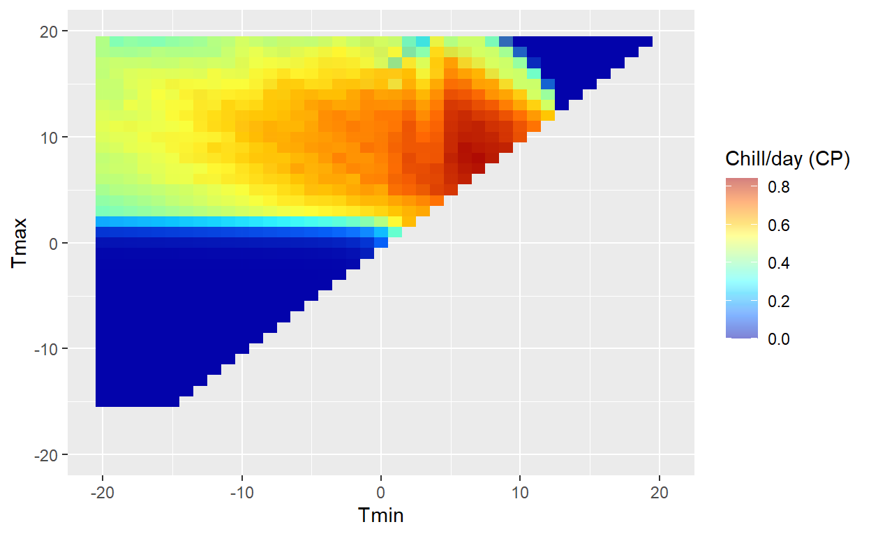
DM_sensitivity <- DM_sensitivity +
  facet_wrap(vars(Month_names)) +
  ylim(min(results$Tmax),
       max(results$Tmax)) +
  ylim(min(results$Tmin),
       max(results$Tmin))

DM_sensitivity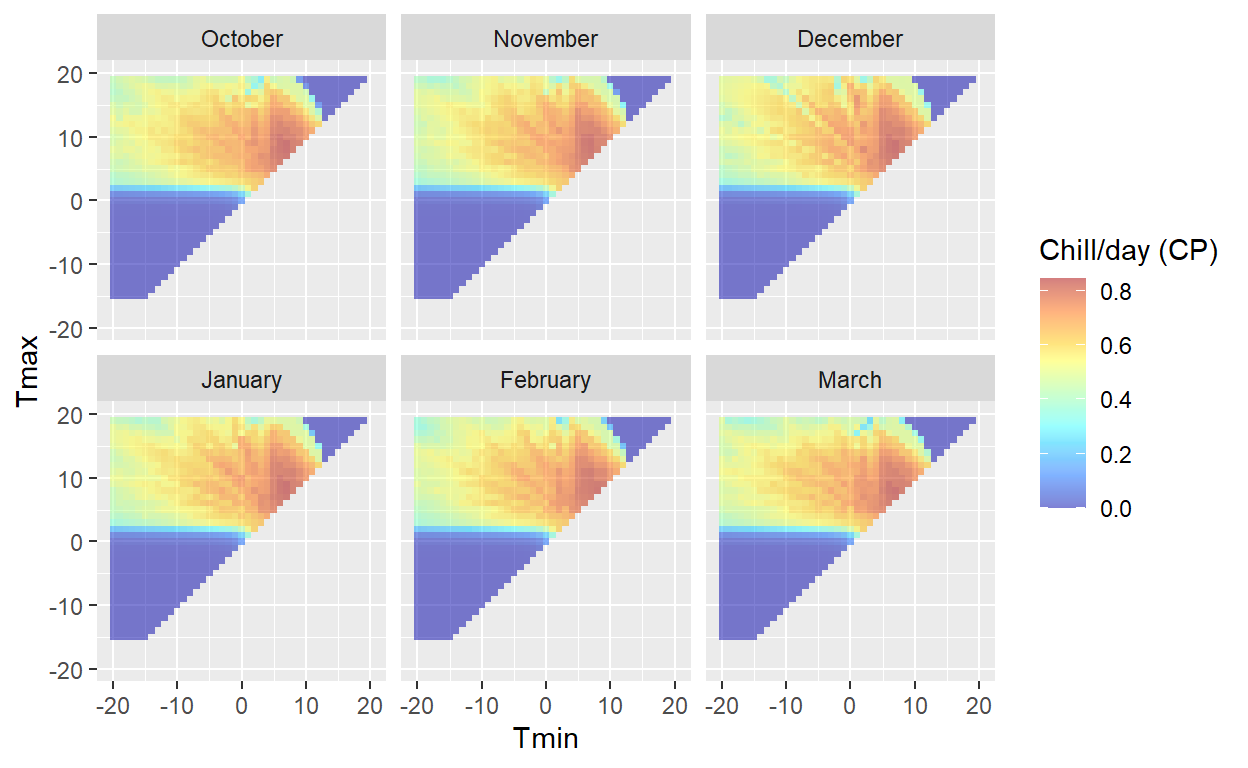
Comparing Locations
To assess the model’s suitability for different climates, temperature data is overlaid on the model sensitivity plot. This enables comparison of temperature response patterns across multiple locations like Klein-Altendorf, Davis, Beijing, and Sfax.
temperatures <- read_tab("data/TMaxTMin1958-2019_patched.csv") %>%
  filter(Month %in% month_range) %>%
  mutate(Month_names =
           factor(Month,
                  levels = c(10, 11, 12, 1, 2, 3),
                  labels = c("October", "November", "December",
                             "January", "February", "March")))

temperatures[which(temperatures$Tmax < temperatures$Tmin),
             c("Tmax", "Tmin")] <- NA

DM_sensitivity +
  geom_point(data = temperatures,
             aes(x = Tmin,
                 y = Tmax,
                 fill = NULL,
                 color = "Temperature"),
             size = 0.2) +
  facet_wrap(vars(Month_names)) +
  scale_color_manual(values = "black",
                     labels = "Daily temperature \nextremes (°C)",
                     name = "Observed at site" ) +
  guides(fill = guide_colorbar(order = 1),
         color = guide_legend(order = 2)) +
  ylab("Tmax (°C)") +
  xlab("Tmin (°C)") +
theme_bw(base_size = 15) 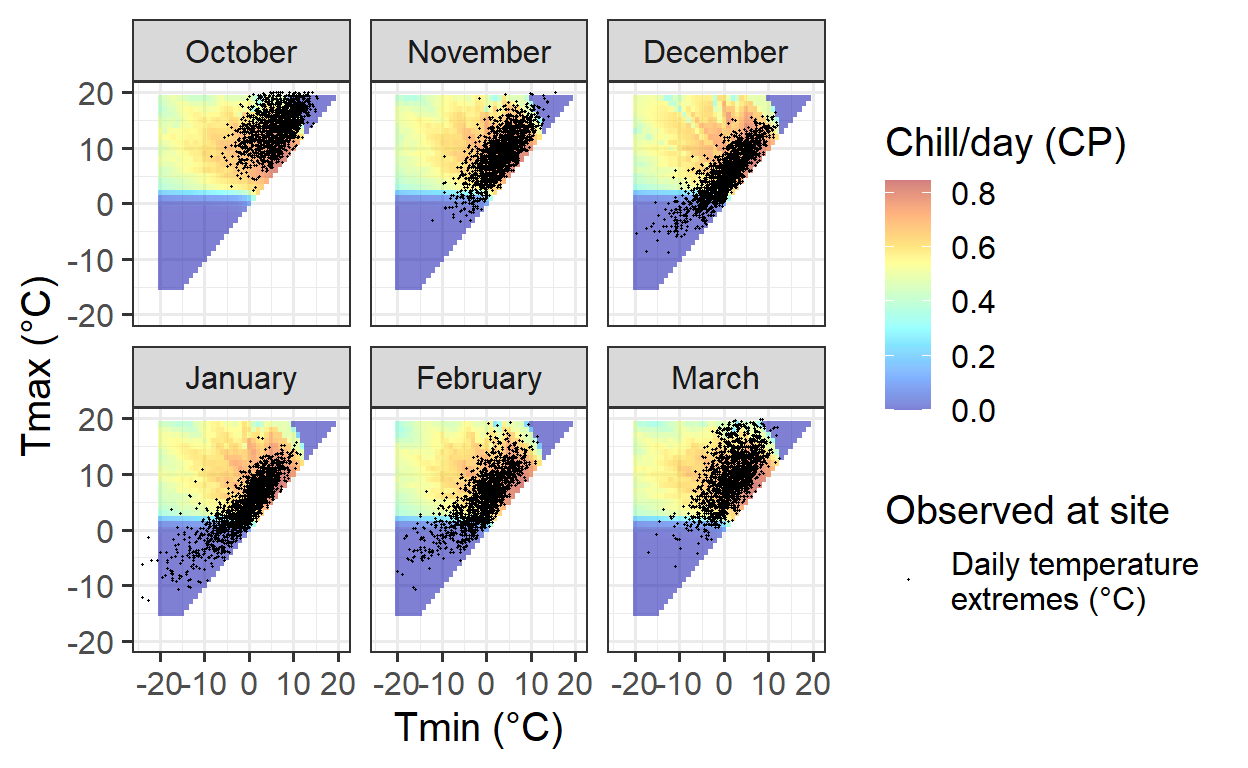
Automating the Process
For efficiency, functions are created to automate model sensitivity calculations and visualizations for various locations. The results are saved to files for easy reuse, making it easier to compare responses across different locations without reprocessing data.
Chill_model_sensitivity <-
  function(latitude,
           temp_models = list(Dynamic_Model = Dynamic_Model,
                              GDH = GDH),
           month_range = c(10, 11, 12, 1, 2, 3),
           Tmins = c(-10:20),
           Tmaxs = c(-5:30))
  {
  mins <- NA
  maxs <- NA
  metrics <- as.list(rep(NA,
                         length(temp_models)))
  names(metrics) <- names(temp_models)
  month <- NA

  for(mon in month_range)
    {
    days_month <-
      as.numeric(difftime(ISOdate(2002,
                                  mon + 1,
                                  1),
                          ISOdate(2002,
                                  mon,
                                  1) ))
    if(mon == 12) days_month <- 31
    weather <-
      make_all_day_table(data.frame(Year = c(2001, 2001),
                                    Month = c(mon, mon),
                                    Day = c(1, days_month),
                                    Tmin = c(0, 0),
                                    Tmax = c(0, 0)))


    for(tmin in Tmins)
      for(tmax in Tmaxs)
        if(tmax >= tmin)
          {
          hourtemps <- weather %>%
            mutate(Tmin = tmin,
                   Tmax = tmax) %>%
            stack_hourly_temps(
              latitude = latitude) %>%
            pluck("hourtemps",
                  "Temp")

          for(tm in 1:length(temp_models))
            metrics[[tm]] <-
              c(metrics[[tm]],
                tail(do.call(temp_models[[tm]],
                        list(hourtemps)),1)/
                              days_month)

          mins <- c(mins, tmin)
          maxs <- c(maxs, tmax)
          month <- c(month, mon)
        }
    }
  results <- cbind(data.frame(Month = month,
                              Tmin = mins,
                              Tmax = maxs),
                   as.data.frame(metrics))

  results <- results[!is.na(results$Month),]
}


Chill_sensitivity_temps <-
  function(chill_model_sensitivity_table,
           temperatures,
           temp_model,
           month_range = c(10, 11, 12, 1, 2, 3),
           Tmins = c(-10:20),
           Tmaxs = c(-5:30),
           legend_label = "Chill/day (CP)")
{

  cmst <- chill_model_sensitivity_table
  cmst <- cmst[which(cmst$Month %in% month_range),]
  cmst$Month_names <- factor(cmst$Month,
                             levels = month_range,
                             labels = month.name[month_range])

  DM_sensitivity<-
    ggplot(cmst,
           aes_string(x = "Tmin",
                      y = "Tmax",
                      fill = temp_model)) +
    geom_tile() +
    scale_fill_gradientn(colours = alpha(matlab.like(15),
                                         alpha = .5),
                         name = legend_label) +
    xlim(Tmins[1],
         Tmins[length(Tmins)]) +
    ylim(Tmaxs[1],
         Tmaxs[length(Tmaxs)])

  temperatures<-
    temperatures[which(temperatures$Month %in% month_range),]

  temperatures[which(temperatures$Tmax < temperatures$Tmin),
               c("Tmax",
                 "Tmin")] <- NA

  temperatures$Month_names <-
    factor(temperatures$Month,
           levels = month_range,
           labels = month.name[month_range])

  DM_sensitivity +
    geom_point(data = temperatures,
               aes(x = Tmin,
                   y = Tmax,
                   fill = NULL,
                   color = "Temperature"),
               size = 0.2) +
    facet_wrap(vars(Month_names)) +
    scale_color_manual(values = "black",
                       labels = "Daily temperature \nextremes (°C)",
                       name = "Observed at site" ) +
    guides(fill = guide_colorbar(order = 1),
           color = guide_legend(order = 2)) +
    ylab("Tmax (°C)") +
    xlab("Tmin (°C)") +
    theme_bw(base_size = 15)

}
Model_sensitivities_CKA <-
Chill_model_sensitivity(latitude = 50,
temp_models = list(Dynamic_Model = Dynamic_Model,
GDH = GDH),
month_range = c(10:12, 1:5))
write.csv(Model_sensitivities_CKA,
"data/Model_sensitivities_CKA.csv",
row.names = FALSE)
Model_sensitivities_Davis <-
Chill_model_sensitivity(latitude = 38.5,
temp_models = list(Dynamic_Model = Dynamic_Model,
GDH = GDH),
month_range=c(10:12, 1:5))
write.csv(Model_sensitivities_Davis,
"data/Model_sensitivities_Davis.csv",
row.names = FALSE)
Model_sensitivities_Beijing <-
Chill_model_sensitivity(latitude = 39.9,
temp_models = list(Dynamic_Model = Dynamic_Model,
GDH = GDH),
month_range = c(10:12, 1:5))
write.csv(Model_sensitivities_Beijing,
"data/Model_sensitivities_Beijing.csv",
row.names = FALSE)
Model_sensitivities_Sfax <-
Chill_model_sensitivity(latitude = 35,
temp_models = list(Dynamic_Model = Dynamic_Model,
GDH = GDH),
month_range = c(10:12, 1:5))
write.csv(Model_sensitivities_Sfax,
"data/Model_sensitivities_Sfax.csv",
row.names = FALSE)Now, temperature patterns for specific months can be compared to the effective ranges for chill and heat accumulation at the four locations. By analyzing long-term weather data, it becomes possible to assess how well each site’s climate aligns with the conditions necessary for dormancy processes.
The analysis will begin with Beijing, the coldest location, and then progress through Klein-Altendorf, Davis, and Sfax, representing increasingly warmer growing regions. This step-by-step approach allows for a clear comparison of chill accumulation across different climates.
Since Chill_sensitivity_temps outputs a ggplot object, it can be modified using the + notation in ggplot2. Titles will be added to each plot using the ggtitle function to improve clarity. Below are the generated plots for chill accumulation, quantified using the Dynamic Model, illustrating how effective temperature ranges vary across these locations.
Chill_sensitivity_temps(Model_sensitivities_Beijing,
                        Beijing_weather,
                        temp_model = "Dynamic_Model",
                        month_range = c(10, 11, 12, 1, 2, 3),
                        legend_label = "Chill per day \n(Chill Portions)") +
  ggtitle("Chill model sensitivity at Beijing, China")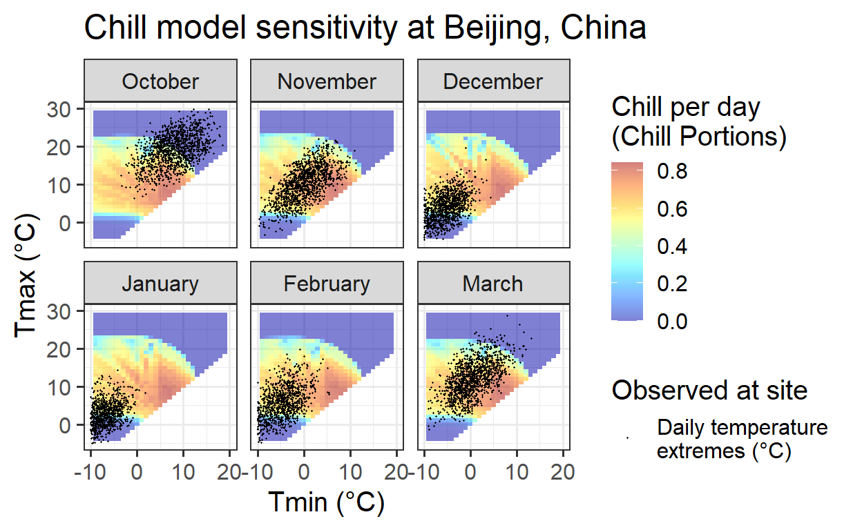
Chill_sensitivity_temps(Model_sensitivities_CKA,
                        CKA_temperatures,
                        temp_model = "Dynamic_Model",
                        month_range = c(10, 11, 12, 1, 2, 3),
                        legend_label = "Chill per day \n(Chill Portions)") +
  ggtitle("Chill model sensitivity at Klein-Altendorf, Germany")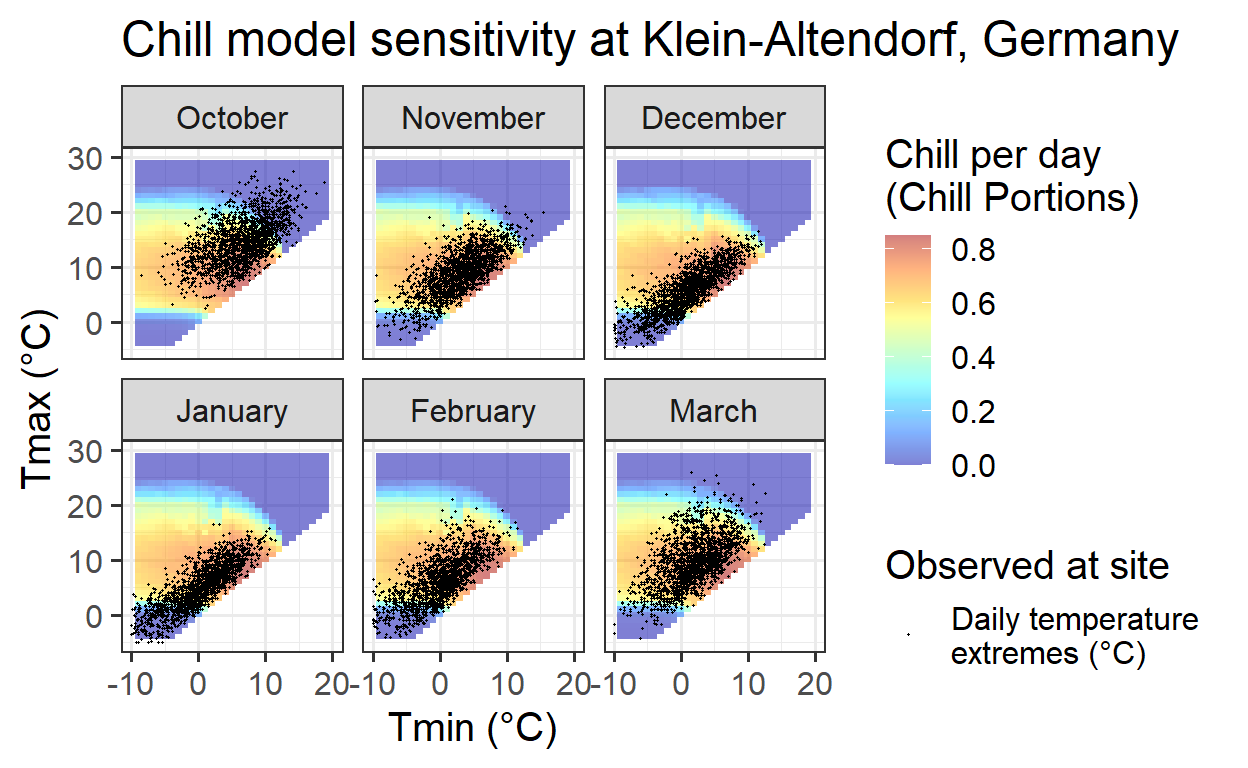
Chill_sensitivity_temps(Model_sensitivities_Davis,
                        Davis_weather,
                        temp_model = "Dynamic_Model",
                        month_range = c(10, 11, 12, 1, 2, 3),
                        legend_label = "Chill per day \n(Chill Portions)") +
  ggtitle("Chill model sensitivity at Davis, California")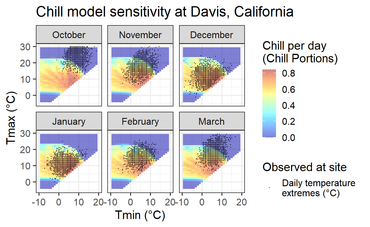
Chill_sensitivity_temps(Model_sensitivities_Sfax,
                        Sfax_weather,
                        temp_model = "Dynamic_Model",
                        month_range = c(10, 11, 12, 1, 2, 3),
                        legend_label = "Chill per day \n(Chill Portions)") +
  ggtitle("Chill model sensitivity near Sfax, Tunisia")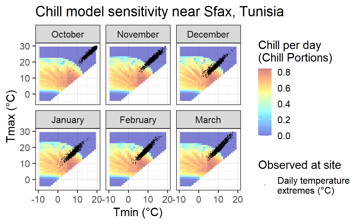
Below are the plots for heat accumulation:
Chill_sensitivity_temps(Model_sensitivities_Beijing,
                        Beijing_weather,
                        temp_model = "GDH",
                        month_range = c(12, 1:5),
                        legend_label = "Heat per day \n(GDH)") +
  ggtitle("Heat model sensitivity at Beijing, China")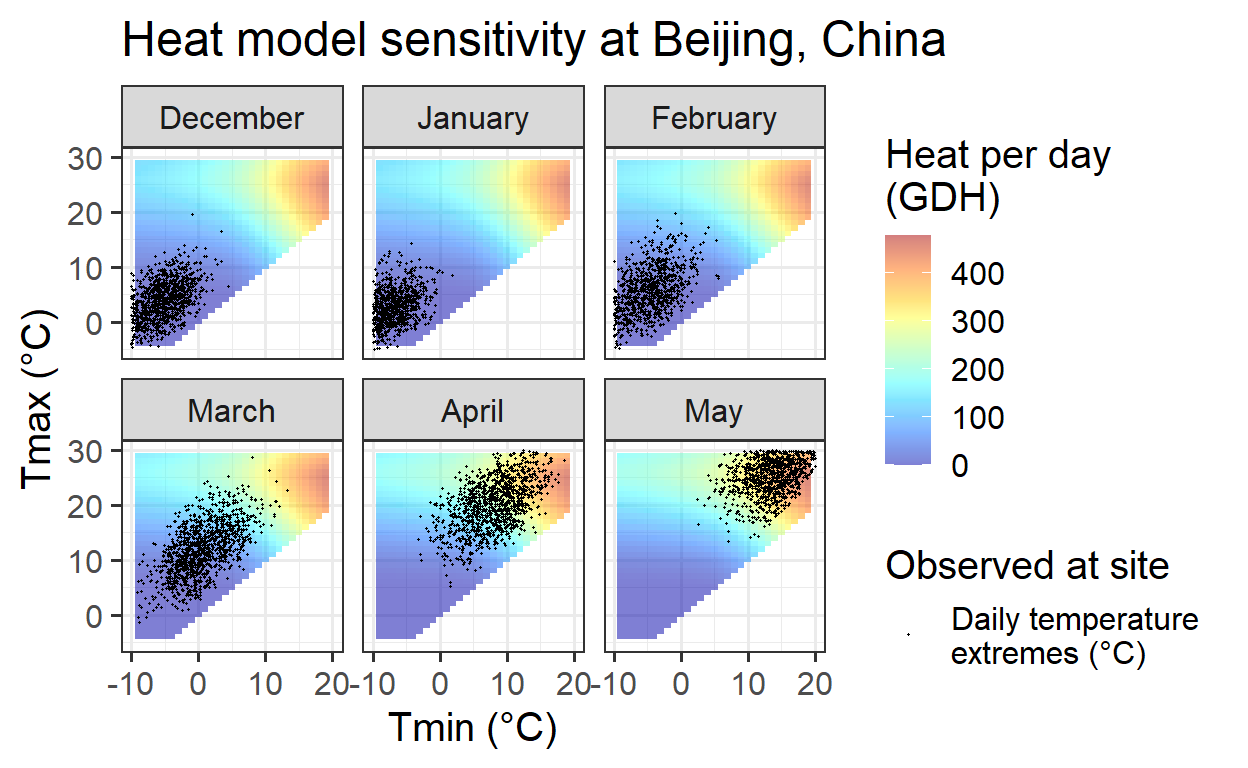
Chill_sensitivity_temps(Model_sensitivities_CKA,
                        CKA_temperatures,
                        temp_model = "GDH",
                        month_range = c(12, 1:5),
                        legend_label = "Heat per day \n(GDH)") +
  ggtitle("Heat model sensitivity at Klein-Altendorf, Germany")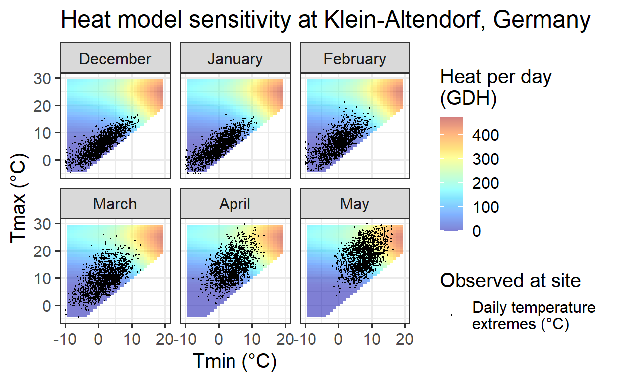
Chill_sensitivity_temps(Model_sensitivities_Davis,
                        Davis_weather,
                        temp_model = "GDH",
                        month_range = c(12, 1:5),
                        legend_label = "Heat per day \n(GDH)") +
  ggtitle("Heat model sensitivity at Davis, California")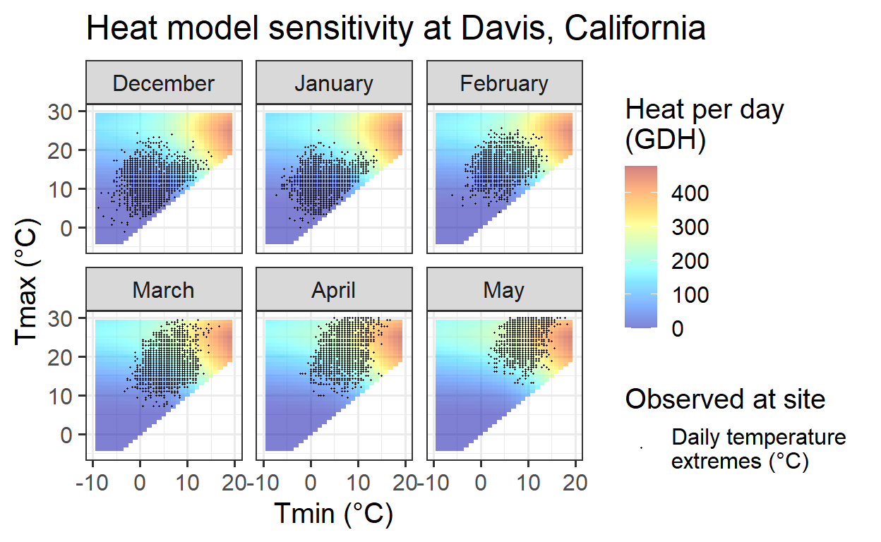
Chill_sensitivity_temps(Model_sensitivities_Sfax,
                        Sfax_weather,
                        temp_model = "GDH",
                        month_range = c(12, 1:5),
                        legend_label = "Heat per day \n(GDH)") +
  ggtitle("Heat model sensitivity near Sfax, Tunisia")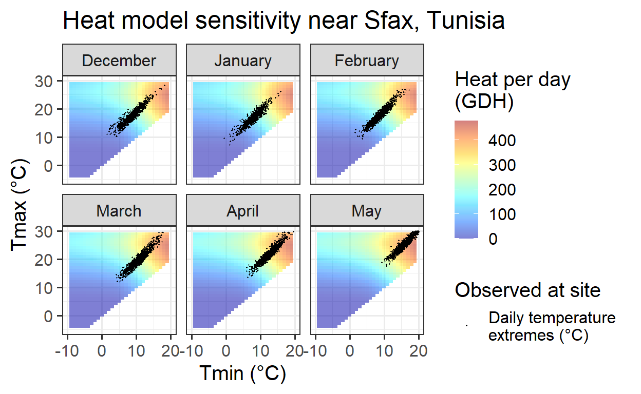
Now, the response patterns will be analyzed in relation to the sensitivity of the chill model. This will help identify how different locations align with the effective temperature ranges for chill accumulation and how variations in climate influence dormancy processes.
Chill model sensitivity vs. observed temperature
Although chill model sensitivity is influenced by hourly temperatures, which depend on sunrise and sunset times, the overall sensitivity patterns appear nearly identical across all locations. While minor differences exist, they are not significant enough to impact the broader interpretation.
What does vary, however, is how observed hourly temperatures align with the sensitive periods for chill accumulation. This alignment shifts not only between locations but also across different months, highlighting the importance of local climatic conditions in determining the effectiveness of chill accumulation.
Beijing, China
In Beijing, the relationship between observed temperatures and effective chill accumulation varies significantly across months:
October: Temperatures are evenly distributed between effective chill accumulation conditions and values that are too warm. This variation may generate chill-related signals, potentially influencing bloom dates in a detectable way.
November: Almost all temperatures fall within the highly effective chill accumulation range. Despite considerable temperature fluctuations, chill accumulation rates remain similar for most days. Without meaningful variation, PLS regression is unlikely to produce useful results.
December–February: Temperatures drop further, leading to many hours below the effective chill accumulation range. If the Dynamic Model correctly represents chill accumulation at low temperatures (which remains uncertain), a response might still be observed.
March: Similar to November, temperatures remain almost always optimal for chill accumulation, resulting in limited variation.
Summary:
Beijing’s conditions should allow for clear identification of chill effects in most months, except for November, where the lack of variation may reduce the effectiveness of PLS regression.
Klein-Altendorf, Germany
Compared to Beijing, Klein-Altendorf appears to be less suitable for using PLS regression to delineate the chilling period. While both locations experience a mix of optimal and suboptimal temperatures, the proportion of days with suboptimal chill conditions is much lower in Klein-Altendorf.
October, December, January, February: Most days have near-optimal chill conditions, with only a few too warm days (mainly in October) or too cold days for effective chill accumulation.
November and March: Almost all days fall within the optimal chill accumulation range, leading to minimal variation.
Summary:
Due to the lack of strong temperature fluctuations, Klein-Altendorf may not be well-suited for PLS regression analysis, as the method relies on meaningful variation to detect temperature response phases.
Davis, California
Davis provides more favorable conditions for PLS regression compared to the colder locations, particularly due to the distribution of daily temperatures across chill model sensitivity levels during certain months.
November and March: Daily temperatures are evenly distributed between effective and ineffective chill accumulation conditions, creating meaningful variation that could help detect temperature response phases.
February: Most days have optimal chill accumulation conditions, with relatively few days experiencing low or zero chill accumulation.
January and December: Conditions are mostly optimal for chill accumulation, with little variation, which may limit PLS regression’s ability to detect meaningful signals.
Summary:
While Davis offers better conditions than colder locations for PLS-based analysis, it may still face limitations, particularly in months where chill accumulation remains consistently high, reducing variability in the data.
Sfax, Tunisia
In Sfax, temperature conditions are generally more favorable for PLS regression, particularly between December and February:
December–February: Temperatures vary enough to create meaningful chill signals, making these months well-suited for PLS-based analysis.
November and March: Some chill accumulation occurs, but the proportion of effective chill days is much lower compared to peak winter months.
October: Temperatures remain consistently too high for chill accumulation, meaning no significant chill-related signal is expected.
Summary:
Among the four locations, Sfax presents the best conditions for PLS regression, especially in mid-winter. However, October shows no variation, and November/March may produce only weak signals, limiting their usefulness in identifying temperature response phases.
Heat model sensitivity vs. observed temperature
Compared to the Dynamic Model, the Growing Degree Hours (GDH) model exhibits a much simpler temperature response. Any day with a minimum temperature above 4°C contributes to heat accumulation, with warmer temperatures leading to a stronger response.
Beijing (December–May): Heat accumulation days are rare in December, January, and February, but become frequent from March onward.
Other locations: Heat accumulation conditions are met in all months, making it easier to detect response phases.
Across the four sites, there are few months where PLS regression would struggle to identify heat accumulation phases. This likely explains why PLS regression has been more effective at detecting ecodormancy (heat accumulation) phases than endodormancy (chill accumulation) periods, where temperature conditions are often more stable and less variable.
Exercises on expected PLS responsiveness
- Produce chill and heat model sensitivity plots for the location you focused on in previous exercises.
# Chill sensitivity model for Yakima
Yakima_weather <- read.csv("Yakima/Yakima_weather.csv")
Model_sensitivities_Yakima <- read.csv("Yakima/Model_sensitivities_Yakima.csv")

Chill_sensitivity_temps(Model_sensitivities_Yakima,
                        Yakima_weather,
                        temp_model = "Dynamic_Model",
                        month_range = c(10, 11, 12, 1, 2, 3),
                        legend_label = "Chill per day \n(Chill Portions)") +
ggtitle("Chill model sensitivity at Yakima, USA") 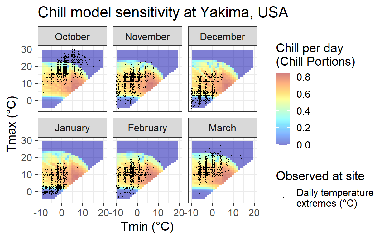
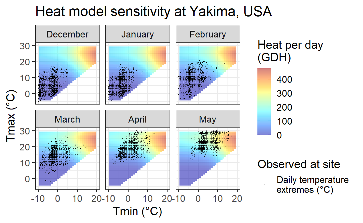
# Heat sensitivity model for Yakima

Chill_sensitivity_temps(Model_sensitivities_Yakima,
                        Yakima_weather,
                        temp_model = "GDH",
                        month_range = c(12, 1:5),
                        legend_label = "Heat per day \n(GDH)") +
  ggtitle("Heat model sensitivity at Yakima, USA")