The Modeling Challenge
Modeling winter chill and predicting budburst dates is complex due to uncertainties in temperature responses, chill accumulation, and heat requirements. These challenges hinder the development of reliable models. While experimental data provide insights into tree responses, including the compensatory effects of heat for low chill, modeling these behaviors remains difficult. A credible model must account for these dynamics to ensure accuracy, and models ignoring key uncertainties or processes lack credibility.
Validating Models
Some models predict bloom dates accurately but may not represent underlying processes. Validation should include output and process validation. Output validation checks prediction accuracy, while process validation compares biological mechanisms in the model with established knowledge. Models must be evaluated within their validity domain, ensuring they are suitable for their intended purpose.
dat <-data.frame(x = c(1, 2, 3, 4),
                y = c(2.3, 2.5, 2.7, 2.7))

ggplot(dat,aes(x = x,
               y = y)) +
  geom_smooth(method = "lm",
              fullrange = TRUE) +
  geom_smooth(method = "lm",
              fullrange = FALSE,
              col = "dark green") +
  geom_point() +
  xlim(c(0,10)) +
  geom_vline(xintercept = 8, col="red") +
  theme_bw(base_size = 15)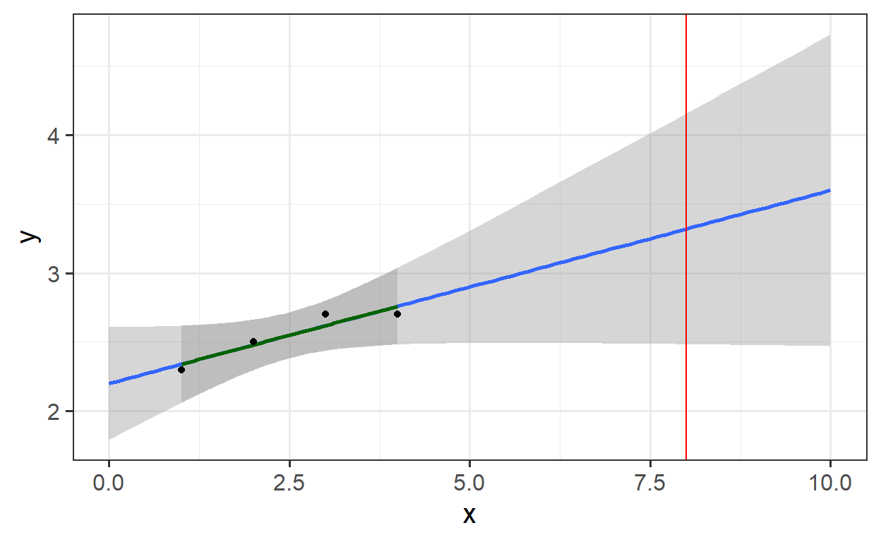
A simple regression model based on data for x-values between 1 and 4 cannot reliably predict y for x=8, as its validity is limited to the range used for calibration. Beyond this range, system behavior is unknown, making extrapolation uncertain. While some might argue that prior knowledge of the system allows for reasonable assumptions about behavior outside the observed range, any such assumption should be explicitly stated and justified.
Mapping validity domains
For complex models like crop or phenology models, defining validity domains is even more difficult, yet often overlooked. Reliable predictions require validation under conditions similar to those the model aims to predict. This is particularly challenging for studies on phenology responses to climate change, where temperature influences may shift over time. Despite this, many models rely on simple equations that fail to account for such changes.
past_weather <- read_tab("data/TMaxTMin1958-2019_patched.csv")
past_weather$SSP_Time <- "Past"

future_temps <- load_temperature_scenarios("data/future_climate",
                                           "Bonn_futuretemps")

SSPs <- c("ssp126", "ssp245", "ssp370", "ssp585")
Times <- c(2050, 2085)

list_ssp <-
  strsplit(names(future_temps), '\\.') %>%
  map(2) %>%
  unlist()

list_gcm <-
  strsplit(names(future_temps), '\\.') %>%
  map(3) %>%
  unlist()

list_time <-
  strsplit(names(future_temps), '\\.') %>%
  map(4) %>%
  unlist()

for(SSP in SSPs)
  for(Time in Times)
   {Temps <- future_temps[list_ssp == SSP & list_time == Time]
    names(Temps) <- list_gcm[list_ssp == SSP & list_time == Time]

    for(gcm in names(Temps))
      Temps[[gcm]] <- Temps[[gcm]] %>%
        mutate(GCM = gcm,
               SSP = SSP,
               Time = Time)

    Temps <- do.call("rbind", Temps)
    if(SSP == SSPs[1] & Time == Times[1])
      results <- Temps else
        results <- rbind(results,
                         Temps)
    }

results$SSP[results$SSP == "ssp126"] <- "SSP1"
results$SSP[results$SSP == "ssp245"] <- "SSP2"
results$SSP[results$SSP == "ssp370"] <- "SSP3"
results$SSP[results$SSP == "ssp585"] <- "SSP5"

results$SSP_Time <- paste0(results$SSP," ",results$Time)

future_months <-
  aggregate(results[, c("Tmin", "Tmax")],
            by = list(results$SSP_Time,
                      results$Year,
                      results$Month),
            FUN = mean)
colnames(future_months)[1:3] <- c("SSP_Time",
                                  "Year",
                                  "Month")

past_months <-
  aggregate(past_weather[, c("Tmin","Tmax")],
            by = list(past_weather$SSP_Time,
                      past_weather$Year,
                      past_weather$Month),
            FUN=mean)
colnames(past_months)[1:3] <- c("SSP_Time", "Year", "Month")

all_months <- rbind(past_months,
                    future_months)

all_months$month_name <- factor(all_months$Month,
                                levels = c(6:12, 1:5),
                                labels = month.name[c(6:12, 1:5)])
Combining Data for Improved Model Coverage
Historical data alone are insufficient for reliable future predictions. Combining past observations with experimentally enhanced data can help expand the model’s validity domain. However, even enhanced observations may not cover all future scenarios, particularly extreme temperature conditions. A combined approach of historical and enhanced data ensures better coverage for reliable phenology forecasts.
enhanced <- read_tab("data/final_weather_data_S1_S2.csv")
enhanced$Year <- enhanced$Treatment
enhanced$SSP_Time <- "Past enhanced"


enhanced_months <- aggregate(enhanced[, c("Tmin", "Tmax")],
                             by = list(enhanced$SSP_Time,
                                       enhanced$Year,
                                       enhanced$Month),
                             FUN = mean)
colnames(enhanced_months)[1:3] <- c("SSP_Time", "Year", "Month")

all_months_enhanced <- rbind(enhanced_months,
                             future_months)

all_months_enhanced$month_name <- factor(all_months_enhanced$Month,
                                         levels = c(6:12, 1:5),
                                         labels = month.name[c(6:12, 1:5)])

# Calculate the hulls for each group
hull_temps_enhanced <- all_months_enhanced %>%
  group_by(SSP_Time,
           month_name) %>%
  slice(chull(Tmin,
              Tmax))

ggplot(hull_temps_enhanced[
  which(hull_temps_enhanced$Month %in% c(10, 11, 12, 1, 2, 3)),],
       aes(Tmin,
           Tmax,
           fill = factor(SSP_Time))) +
  geom_polygon() +
  facet_wrap(vars(month_name)) +
  scale_fill_manual(name="Scenario",
                    breaks=c("Past enhanced",
                             "SSP1 2050",
                             "SSP1 2085",
                             "SSP2 2050",
                             "SSP2 2085",
                             "SSP3 2050",
                             "SSP3 2085",
                             "SSP5 2050",
                             "SSP5 2085"),
                    values=c("black",
                             alpha("light green",0.4),
                             alpha("dark green",0.4),
                             alpha("coral",0.4),
                             alpha("dark red",0.4),
                             alpha("yellow",0.4),
                             alpha("orange",0.4),
                             alpha("light blue",0.4),
                             alpha("dark blue",0.4))) +
  theme_bw(base_size = 15)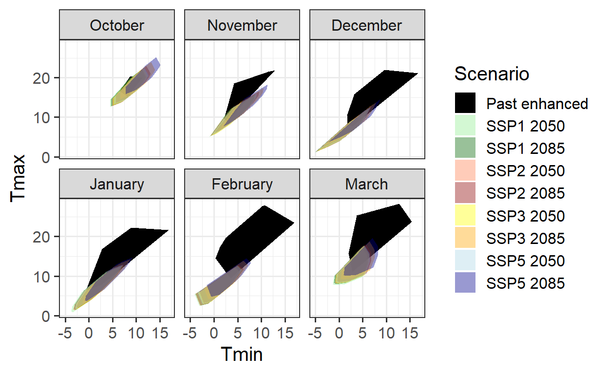
One Last Thought on Model Validity
While phenology models are straightforward, models for crops and other systems are more complex, considering factors like pest management, soil types, and farming methods. Applying these models to diverse agricultural systems, especially smallholder farms, can be problematic and should be done with caution, as they may not accurately represent real-world conditions.
past_months$SSP_Time <- "Past combined"
enhanced_months$SSP_Time <- "Past combined"

all_months_both <- rbind(enhanced_months,
                         past_months,
                         future_months)

all_months_both$month_name <- factor(all_months_both$Month,
                                     levels = c(6:12, 1:5),
                                     labels = month.name[c(6:12, 1:5)])

hull_temps_both <- all_months_both %>%
  group_by(SSP_Time,
           month_name) %>%
  slice(chull(Tmin,
              Tmax))

ggplot(hull_temps_both[
  which(hull_temps_both$Month %in% c(10, 11, 12, 1, 2, 3)),],
       aes(Tmin,
           Tmax,
           fill = factor(SSP_Time))) +
  geom_polygon() +
  facet_wrap(vars(month_name)) +
  scale_fill_manual(name="Scenario",
                    breaks=c("Past combined",
                             "SSP1 2050",
                             "SSP1 2085",
                             "SSP2 2050",
                             "SSP2 2085",
                             "SSP3 2050",
                             "SSP3 2085",
                             "SSP5 2050",
                             "SSP5 2085"),
                    values=c("black",
                             alpha("light green",0.4),
                             alpha("dark green",0.4),
                             alpha("coral",0.4),
                             alpha("dark red",0.4),
                             alpha("yellow",0.4),
                             alpha("orange",0.4),
                             alpha("light blue",0.4),
                             alpha("dark blue",0.4))) +
  theme_bw(base_size = 15)
Exercises on making valid tree phenology models
- Explain the difference between output validation and process validation.
Output validation and process validation assess model reliability in different ways. Output validation checks whether a model accurately predicts observed data using statistical measures like RMSE. However, this does not ensure that the model’s internal processes are correctly represented—it may produce accurate results for the wrong reasons.
Process validation, in contrast, examines whether the model’s mechanisms align with real-world processes. This requires domain knowledge and ensures that key dynamics, such as temperature responses in phenology models, are properly captured. While harder to quantify, process validation is essential for applying models to new conditions.
The main difference is that output validation focuses on predictive accuracy, while process validation ensures that the model’s structure reflects reality.
- Explain what a validity domain is and why it is important to consider this whenever we want to use our model to forecast something.
A validity domain defines the range of conditions under which a model produces reliable results. If used outside this range, predictions may be inaccurate.
Considering the validity domain is crucial for forecasting, as models based on past data may not perform well under new conditions. Applying a model beyond its tested limits without validation increases the risk of misleading conclusions. To ensure reliability, predictions should stay within the model’s validated range or the model should be refined with additional data.
- What is validation for purpose?
Validation for purpose ensures a model is suitable for its intended use. It checks whether the model has been tested under relevant conditions and captures key processes. A model may perform well on past data but still be unreliable for future forecasts if conditions change. This approach prevents misapplication and ensures meaningful predictions.
- How can we ensure that our model is suitable for the predictions we want to make?
To ensure a model is suitable for predictions, we must:
Define the Purpose – Clearly identify what the model should predict and under what conditions.
Check the Validity Domain – Ensure the model has been tested under conditions similar to those it will be applied to.
Validate Both Output and Process – Confirm that predictions match observed data (output validation) and that the model correctly represents real-world processes (process validation).
Assess Uncertainty – Identify possible errors and quantify uncertainties in the predictions.
Refine with Additional Data – Expand or adjust the model using experimental or new observational data to improve its reliability.