Jacqueline Wingen: Filling gaps in temperature records

Weather data often contains gaps due to equipment malfunctions, power outages, or storage problems. These gaps create challenges for modeling agroclimatic conditions, requiring effective gap-filling methods.

Filling Short Gaps in Daily Records

For short gaps (2-3 days), linear interpolation estimates missing values by averaging the last known and first known values around the gap. The chillR package provides the interpolate_gaps() function for this:

weather <- KA_weather %>% make_all_day_table()

Tmin_int <- interpolate_gaps(weather[,"Tmin"])
weather <- weather %>% mutate(Tmin = Tmin_int$interp, Tmin_interpolated = Tmin_int$missing)

Tmax_int <- interpolate_gaps(weather[,"Tmax"])
weather <- weather %>% mutate(Tmax = Tmax_int$interp, Tmax_interpolated = Tmax_int$missing)

KA_weather_gap <- rbind(KA_weather, c(Year = 2011,
                                      Month = 3,
                                      Day = 3,
                                      Tmax = 26,
                                      Tmin = 14))

The fix_weather() function can also be used to fill gaps:

fixed_winter_days <- KA_weather_gap %>% fix_weather(start_year = 2000, 
                                                    end_year = 2011, 
                                                    start_date = 300, 
                                                    end_date = 100)
fixed_all_days <- KA_weather_gap %>% fix_weather()

The function returns a weather dataframe with interpolated data and a QC object summarizing interpolation quality:

fixed_winter_days$QC

Season	End_year	Season_days	Data_days	Missing_Tmin	Missing_Tmax	Incomplete_days	Perc_complete
1999/2000	2000	166	100	66	66	66	60.2
2000/2001	2001	167	167	0	0	0	100.0
2001/2002	2002	166	166	0	0	0	100.0
2002/2003	2003	166	166	0	0	0	100.0
2003/2004	2004	166	166	0	0	0	100.0
2004/2005	2005	167	167	0	0	0	100.0
2005/2006	2006	166	166	0	0	0	100.0
2006/2007	2007	166	166	0	0	0	100.0
2007/2008	2008	166	166	0	0	0	100.0
2008/2009	2009	167	167	0	0	0	100.0
2009/2010	2010	166	166	0	0	0	100.0
2010/2011	2011	166	128	165	165	165	0.6

fixed_all_days$QC

Season	End_year	Season_days	Data_days	Missing_Tmin	Missing_Tmax	Incomplete_days	Perc_complete
1997/1998	1998	365	365	0	0	0	100.0
1998/1999	1999	365	365	0	0	0	100.0
1999/2000	2000	366	366	0	0	0	100.0
2000/2001	2001	365	365	0	0	0	100.0
2001/2002	2002	365	365	0	0	0	100.0
2002/2003	2003	365	365	0	0	0	100.0
2003/2004	2004	366	366	0	0	0	100.0
2004/2005	2005	365	365	0	0	0	100.0
2005/2006	2006	365	365	0	0	0	100.0
2006/2007	2007	365	365	0	0	0	100.0
2007/2008	2008	366	366	0	0	0	100.0
2008/2009	2009	365	365	0	0	0	100.0
2009/2010	2010	365	365	214	214	214	41.4
2010/2011	2011	365	62	364	364	364	0.3

A plot illustrates the effect of gap length on interpolation accuracy:

gap_weather <- KA_weather[200:305, ]
gap_weather[ ,"Tmin_observed"] <- gap_weather$Tmin
gap_weather$Tmin[c(2, 4:5, 7:9, 11:14, 16:20, 22:27, 29:35, 
                   37:44, 46:54, 56:65, 67:77, 79:90, 92:104)] <- NA
fixed_gaps <- fix_weather(gap_weather)$weather

ggplot(data = fixed_gaps, aes(DATE, Tmin_observed)) +
  geom_line(lwd = 1.3) +
  xlab("Date") +
  ylab("Daily minimum temperature (°C)") +
  geom_line(data = fixed_gaps, aes(DATE, Tmin), col = "red", lwd = 1.3)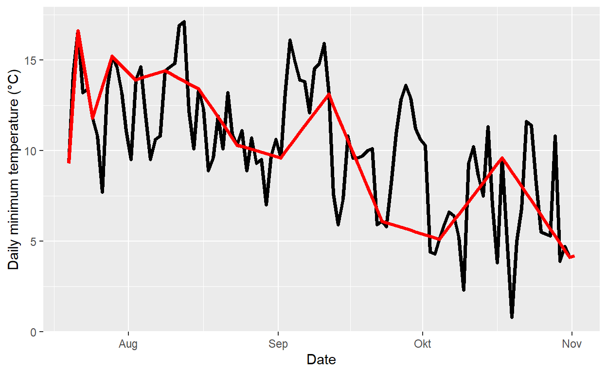

Interpolation errors increase with gap size:

fixed_gaps[,"error"] <- abs(fixed_gaps$Tmin - fixed_gaps$Tmin_observed)

ggplot(data = fixed_gaps, aes(DATE, error)) +
  geom_line(lwd = 1.3) +
  xlab("Date") +
  ylab("Error introduced by interpolation (°C)") +
  geom_point(data = fixed_gaps[which(!fixed_gaps$no_Tmin),], aes(DATE, error), col = "red", cex = 3)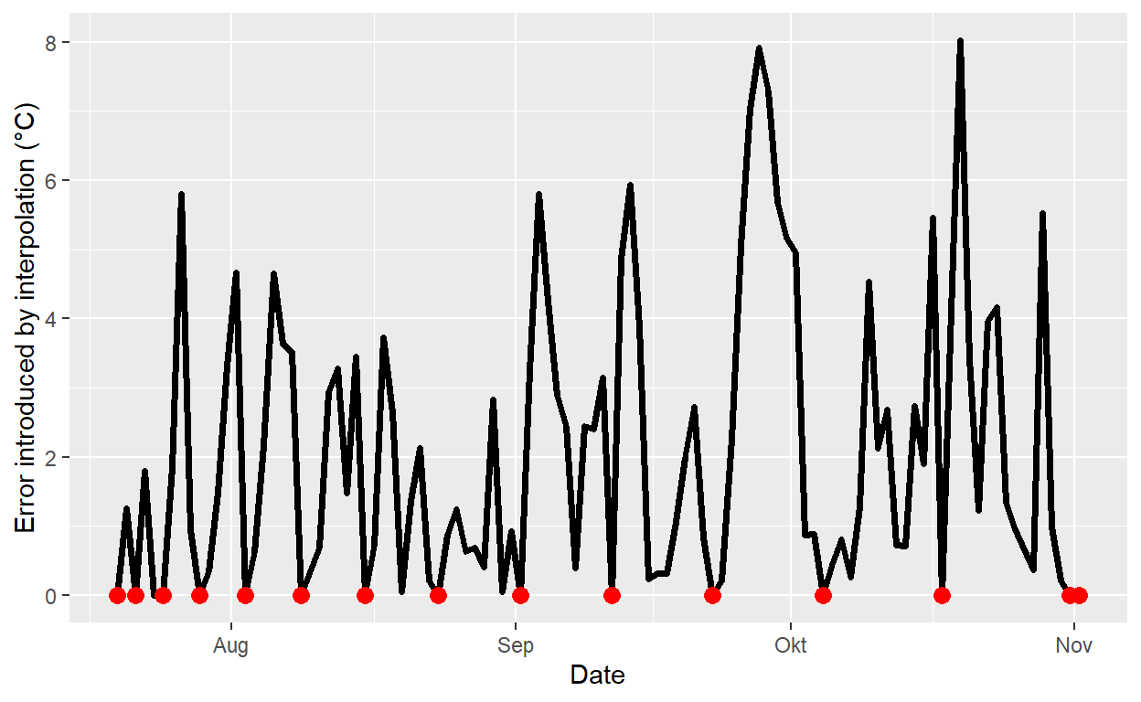

Filling Long Gaps in Daily Records

For long gaps, data from nearby weather stations is used. The patch_weather() function in chillR helps with this:

station_list <- handle_gsod(action = "list_stations",
                            location = c(7.10, 50.73),
                            time_interval = c(1990, 2020))

Relevant stations are downloaded:

patch_weather <- 
  handle_gsod(action = "download_weather", 
              location = as.character(station_list$chillR_code[c(2, 3, 6)]), 
              time_interval = c(1990, 2020)) %>% 
  handle_gsod()

Gaps are filled using patch_daily_temperatures():

patched <- patch_daily_temperatures(weather = Bonn, patch_weather = patch_weather)

Patch statistics are examined:

patched$statistics[[1]]

	mean_bias	stdev_bias	filled	gaps_remain
Tmin	-0.307	1.304	2146	1
Tmax	0.202	1.154	2146	1

patched$statistics[[2]]

	mean_bias	stdev_bias	filled	gaps_remain
Tmin	-1.871	2.080	0	1
Tmax	1.466	1.427	0	1

patched$statistics[[3]]

	mean_bias	stdev_bias	filled	gaps_remain
Tmin	-0.546	1.186	0	1
Tmax	1.314	1.089	0	1

To improve accuracy, mean bias and standard deviation bias limits are set:

patched <- patch_daily_temperatures(weather = Bonn, 
                                    patch_weather = patch_weather, 
                                    max_mean_bias = 1, 
                                    max_stdev_bias = 2)

Final gaps are identified:

post_patch_stats <- fix_weather(patched)$QC

Remaining short gaps are filled with interpolation:

Bonn_weather <- fix_weather(patched)

For seasonally adjusted bias correction, patch_daily_temps() is used:

patched_monthly <- patch_daily_temps(weather = Bonn, 
                                     patch_weather = patch_weather, 
                                     max_mean_bias = 1, 
                                     max_stdev_bias = 2, 
                                     time_interval = "month")

This function allows for interval-based bias corrections:

patched_2weeks <- patch_daily_temps(weather = Bonn, 
                                    patch_weather = patch_weather, 
                                    max_mean_bias = 1, 
                                    max_stdev_bias = 2, 
                                    time_interval = "2 weeks")

Using finer time intervals improves bias correction accuracy, but requires sufficient data for reliability.

`Exercises` on filling gaps

Use chillR functions to find out how many gaps you have in your dataset (even if you have none, please still follow all further steps)

Yakima <- read.csv("Yakima/Yakima_chillR_weather.csv")
Yakima_QC <- fix_weather(Yakima)$QC

Season	End_year	Season_days	Data_days	Perc_complete
1989/1990	1990	365	365	100
1990/1991	1991	365	365	100
1991/1992	1992	366	366	100
1992/1993	1993	365	365	100
1993/1994	1994	365	365	100
1994/1995	1995	365	365	100
1995/1996	1996	366	366	100
1996/1997	1997	365	365	100
1997/1998	1998	365	365	100
1998/1999	1999	365	365	100
1999/2000	2000	366	366	100
2000/2001	2001	365	365	100
2001/2002	2002	365	365	100
2002/2003	2003	365	365	100
2003/2004	2004	366	366	100
2004/2005	2005	365	365	100
2005/2006	2006	365	365	100
2006/2007	2007	365	365	100
2007/2008	2008	366	366	100
2008/2009	2009	365	365	100
2009/2010	2010	365	365	100
2010/2011	2011	365	365	100
2011/2012	2012	366	366	100
2012/2013	2013	365	365	100
2013/2014	2014	365	365	100
2014/2015	2015	365	365	100
2015/2016	2016	366	366	100
2016/2017	2017	365	365	100
2017/2018	2018	365	365	100
2018/2019	2019	365	365	100
2019/2020	2020	366	366	100

Create a list of the 25 closest weather stations using the handle_gsod function

station_list_Yakima <- handle_gsod(action = "list_stations",
                                   location = c(long = -120.50, lat = 46.60),
                                   time_interval = c(1990, 2020))

chillR_code	STATION.NAME	CTRY	Lat	Long	BEGIN	END	Distance	Overlap_years	Perc_interval_covered
72781024243	YAKIMA AIR TERMINAL/MCALSR FIELD AP	US	46.564	-120.535	19730101	20250304	4.82	31.00	100
99999924243	YAKIMA AIR TERMINAL	US	46.568	-120.543	19480101	19721231	4.85	0.00	0
72781399999	VAGABOND AAF / YAKIMA TRAINING CENTER WASHINGTON USA	US	46.667	-120.454	20030617	20081110	8.25	5.40	17
72056299999	RANGE OP 13 / YAKIMA TRAINING CENTER	US	46.800	-120.167	20080530	20170920	33.79	9.31	30
72788399999	BOWERS FLD	US	47.033	-120.531	20000101	20031231	48.26	4.00	13
72788324220	BOWERS FIELD AIRPORT	US	47.034	-120.531	19880106	20250304	48.37	31.00	100
99999924220	ELLENSBURG BOWERS FI	US	47.034	-120.530	19480601	19550101	48.37	0.00	0
72784094187	HANFORD AIRPORT	US	46.567	-119.600	20060101	20130326	68.96	7.23	23
72784099999	HANFORD	US	46.567	-119.600	19730101	19971231	68.96	8.00	26
72782594239	PANGBORN MEMORIAL AIRPORT	US	47.397	-120.201	20000101	20250304	91.58	21.00	68
72782599999	PANGBORN MEM	US	47.399	-120.207	19730101	19971231	91.69	8.00	26
72788499999	RICHLAND AIRPORT	US	46.306	-119.304	19810203	20250303	97.39	31.00	100
72781524237	STAMPASS PASS FLTWO	US	47.277	-121.337	19730101	20250304	98.63	31.00	100
99999924237	STAMPEDE PASS	US	47.277	-121.337	19480101	19721231	98.63	0.00	0
72790024141	EPHRATA MUNICIPAL AIRPORT	US	47.308	-119.516	20050101	20250304	108.64	16.00	52
72782624141	EPHRATA MUNICIPAL	US	47.308	-119.515	19420101	19971231	108.69	8.00	26
99999924141	EPHRATA AP FCWOS	US	47.308	-119.515	19480101	19550101	108.69	0.00	0
72782724110	GRANT COUNTY INTL AIRPORT	US	47.193	-119.315	19430610	20250304	111.73	31.00	100
72782799999	MOSES LAKE/GRANT CO	US	47.200	-119.317	20000101	20031231	112.06	4.00	13
72784524163	TRI-CITIES AIRPORT	US	46.270	-119.118	19730101	20250304	112.21	31.00	100
72784599999	TRI CITIES	US	46.267	-119.117	20000101	20031231	112.40	4.00	13
99999924163	PASCO NAS	US	46.267	-119.117	19450401	19460601	112.40	0.00	0
72698824219	MUNICIPAL AIRPORT	US	45.619	-121.166	19730101	20250304	120.70	31.00	100
99999924219	THE DALLES MUNICIPAL ARPT	US	45.619	-121.166	19480101	19650101	120.70	0.00	0
72688399999	HERMISTON MUNI	US	45.828	-119.259	19980514	20051231	128.55	7.64	25

Identify suitable weather stations for patching gaps
Download weather data for promising stations, convert them to chillR format and compile them in a list

patch_weather <-
  handle_gsod(action = "download_weather",
              location = as.character(station_list_Yakima$chillR_code[c(4, 6, 8)]),
              time_interval = c(1990, 2020)) %>%
  handle_gsod()

Use the patch_daily_temperatures function to fill gaps

patched <- patch_daily_temperatures(weather = Yakima,
                                    patch_weather = patch_weather)

# Patch statistics for YRANGE OP 13 /AKIMA TRAINING CENTER
patched$statistics[[1]]

	mean_bias	stdev_bias	filled	gaps_remain
Tmin	NA	NA	NA	NA
Tmax	NA	NA	NA	NA

# Patch statistics for HANFORD AIRPORT
patched$statistics[[2]]

	mean_bias	stdev_bias	filled	gaps_remain
Tmin	NA	NA	NA	NA
Tmax	NA	NA	NA	NA

# Patch statistics for BOWERS FIELD AIRPORT
patched$statistics[[3]]

	mean_bias	stdev_bias	filled	gaps_remain
Tmin	NA	NA	NA	NA
Tmax	NA	NA	NA	NA

Investigate the results - have all gaps been filled?

write.csv(patched$weather,
          "Yakima/Yakima_weather.csv", row.names = FALSE)

Filling gaps in temperature records

Filling Short Gaps in Daily Records

Filling Long Gaps in Daily Records

Exercises on filling gaps

`Exercises` on filling gaps