PLS regression across species and agroclimatic contexts
Since 2012, PLS regression with agroclimatic metrics (chill and heat) has been applied in various contexts. While some researchers have adopted this approach, this chapter focuses on studies involving the author.
Chestnut, jujube and apricot in Beijing
One of the coldest locations where this approach was applied is Beijing, where research led by Guo Liang used bloom data for Chinese chestnut (Castanea mollissima) and jujube (Ziziphus jujuba) to define chilling and forcing periods (Guo Liang et al., 2014). Another study analyzed datasets for apricot (Prunus armeniaca) and mountain peach (Prunus davidiana), yielding the following results:
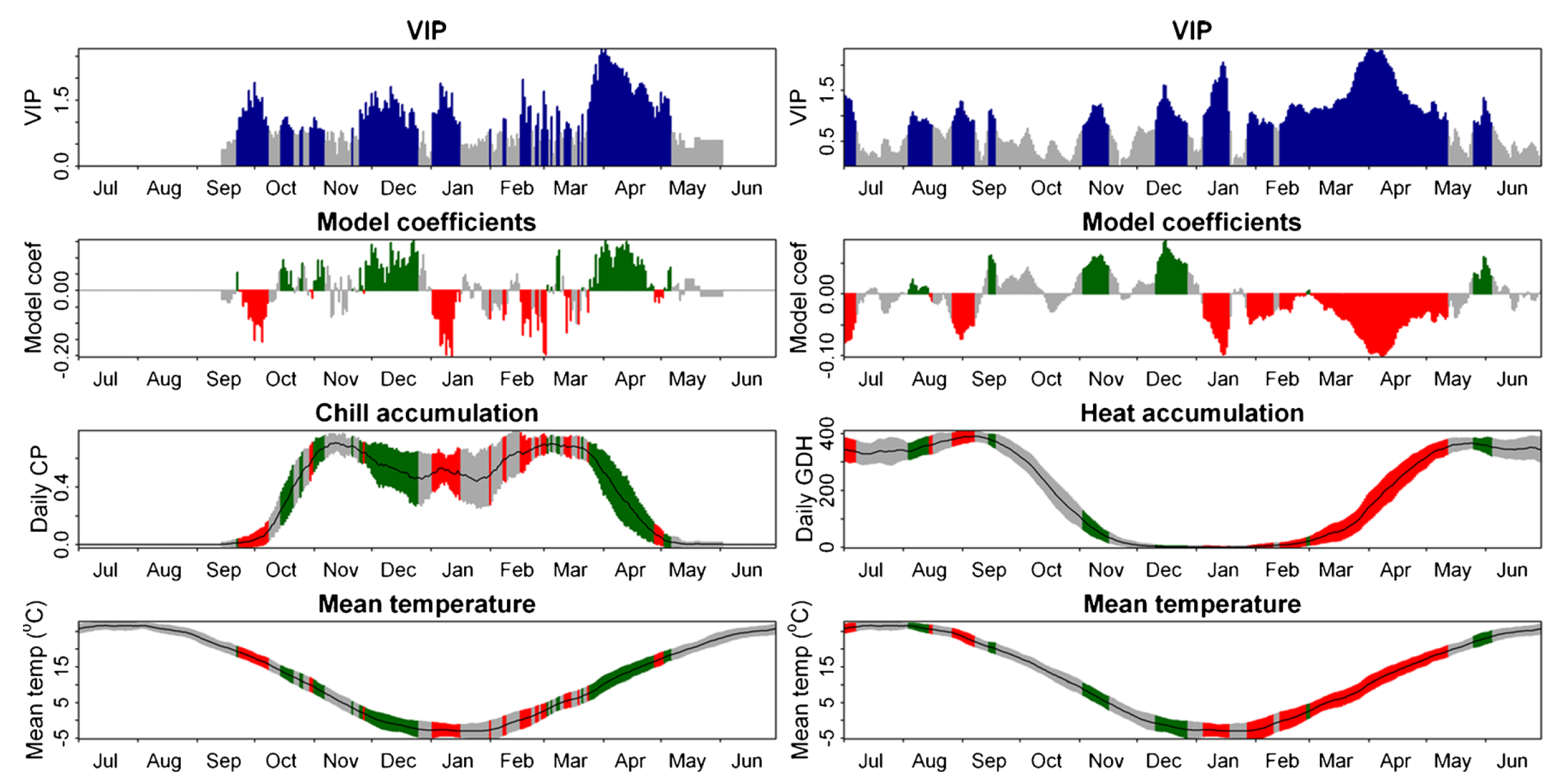
For apricots, PLS regressions were conducted using multiple chill metrics, including Chilling Hours, the Utah Model (Chill Units), and the Dynamic Model (Chill Portions):
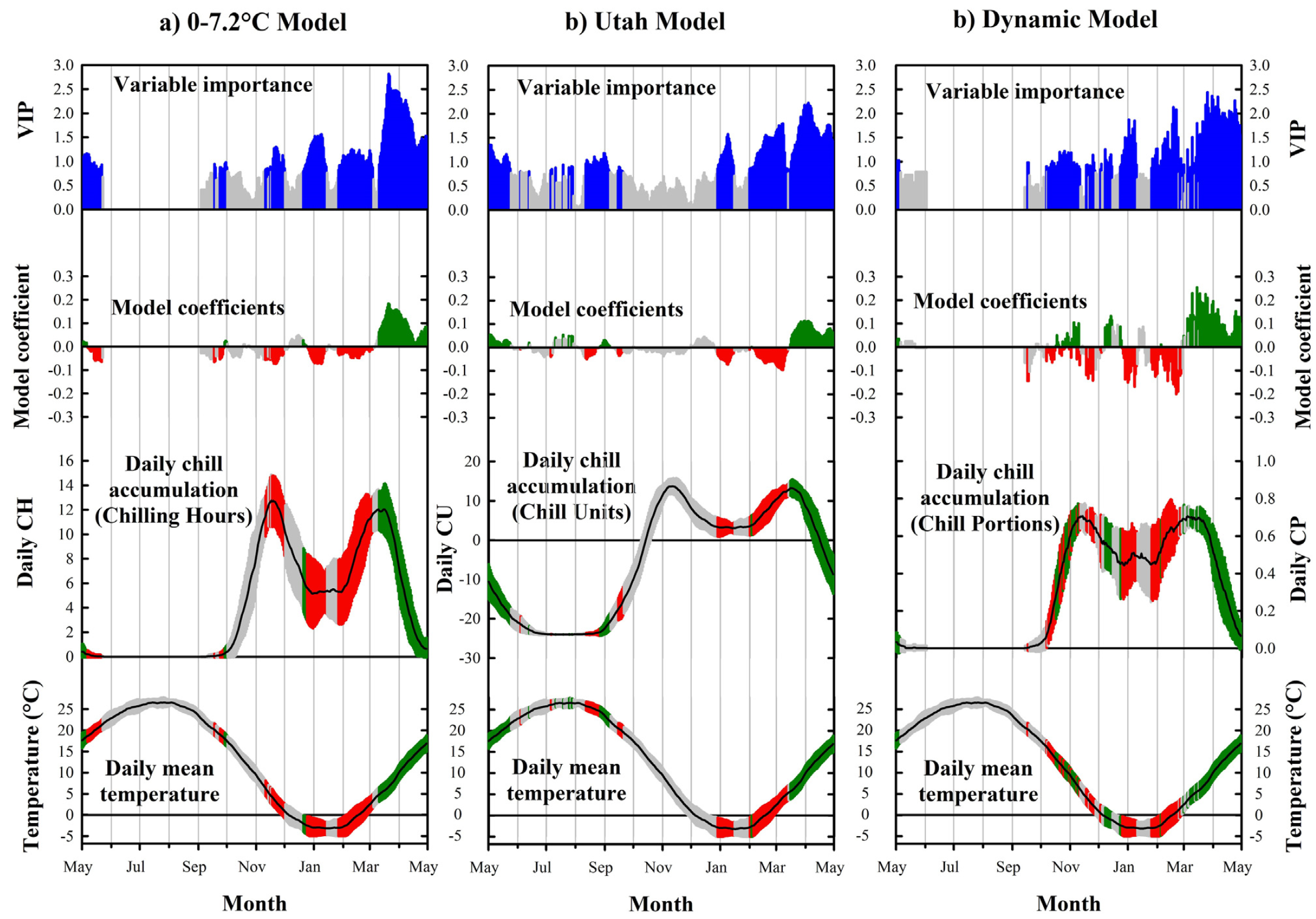
In all analyses of phenology records from Beijing, the forcing period was easy to delineate, but the chilling period was difficult to see.
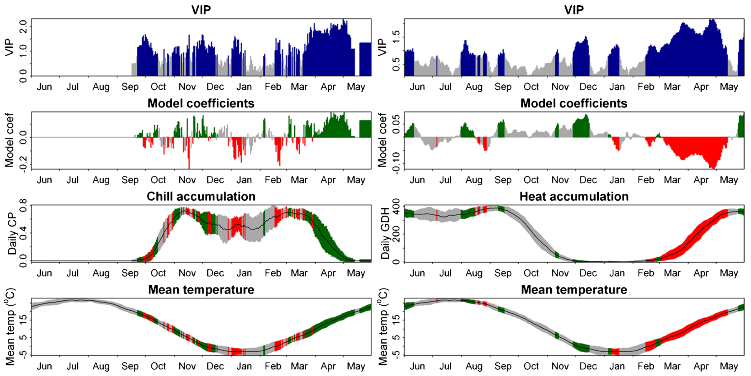
Apples in Shaanxi Province, China
Guo Liang also led a study on apple phenology in Shaanxi, one of China’s main apple growing provinces:
Also here the chilling phase was visible but difficult to delineate.
Cherries in Klein-Altendorf
Winters in Beijing and Shaanxi are quite cold. A slightly warmer location was analyzed by studying cherries in Klein-Altendorf.
Again, it’s pretty difficult to see the chilling period.
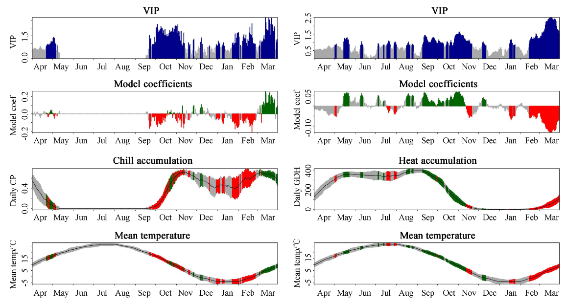
Apricots in the UK
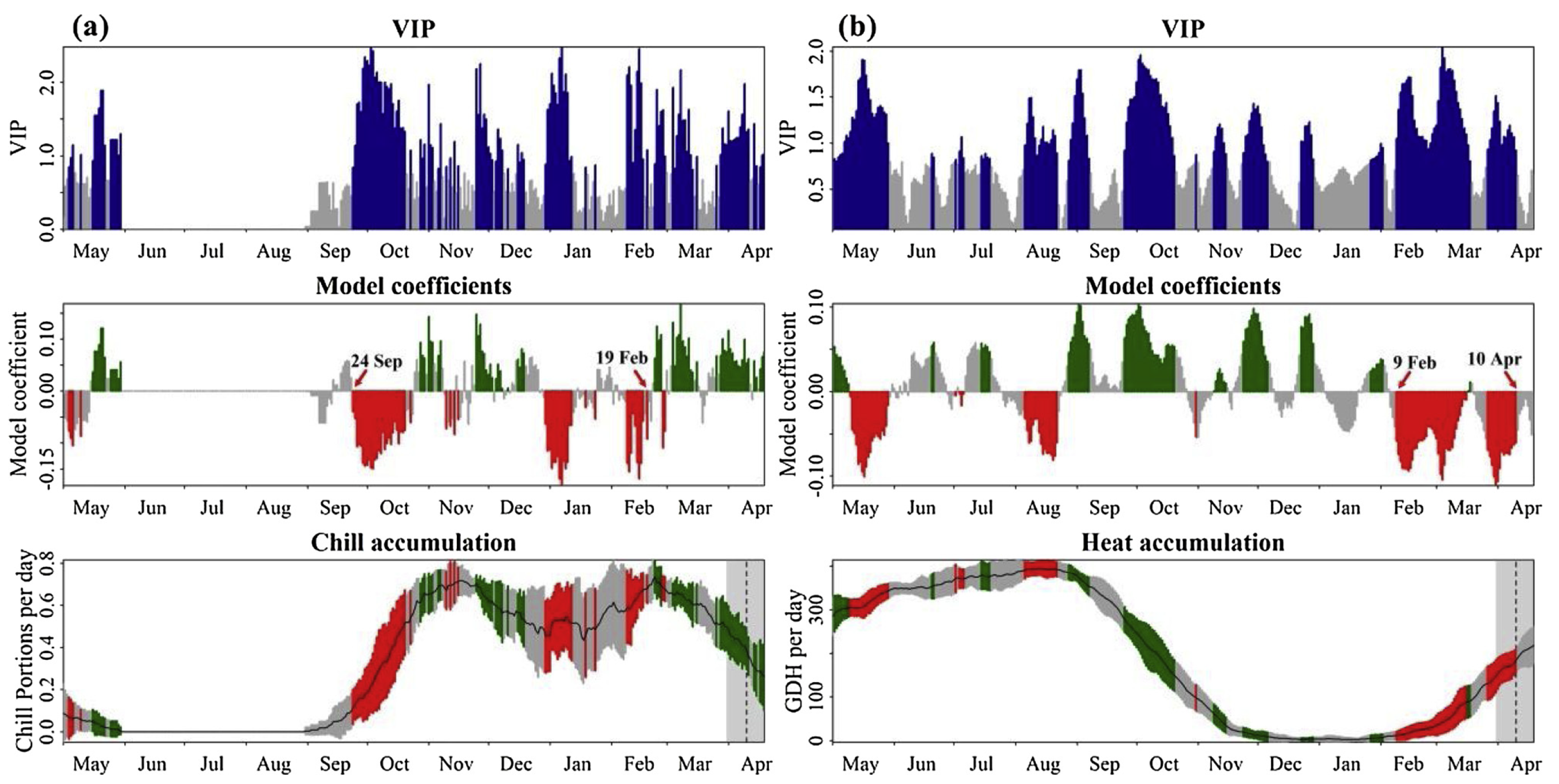
For apricots in the UK National Fruit Collection at Brogdale Farm, Faversham, a clear chill response phase was observed in January and February. However, this period begins later than the typical expected start of chill accumulation.
Grapevine in Croatia
Grapes also have chilling requirements. Johann Johann Martínez-Lüscher, who led the UK apricot study, analyzed the temperature response of grapes grown in Croatia.
In Croatia, where winters are warmer and chill accumulation rates are more variable, the chilling period is more distinct. Bloom response to chill is particularly strong in December and January. With a broader interpretation, the chilling period could extend from late September to February.
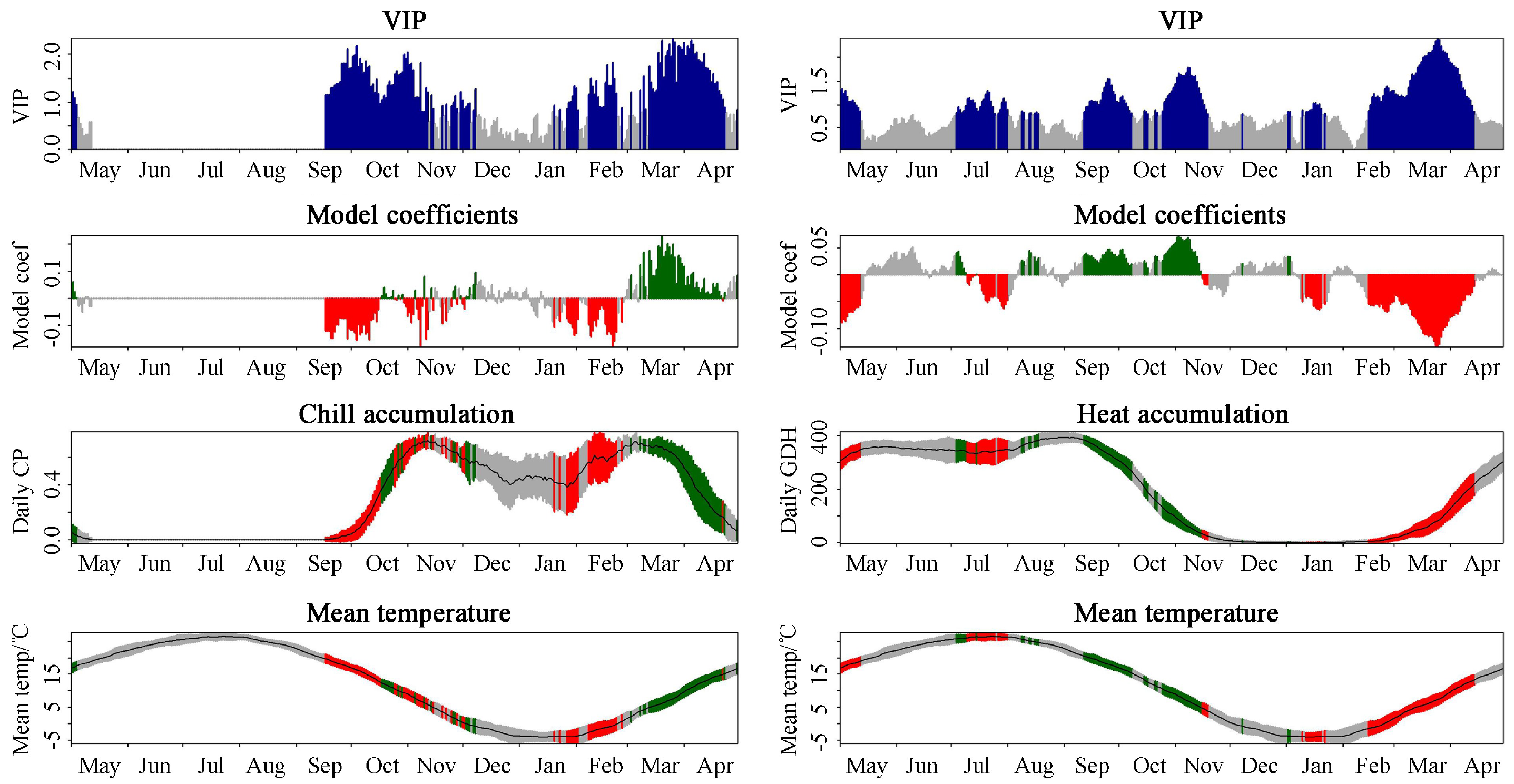
Walnuts in California
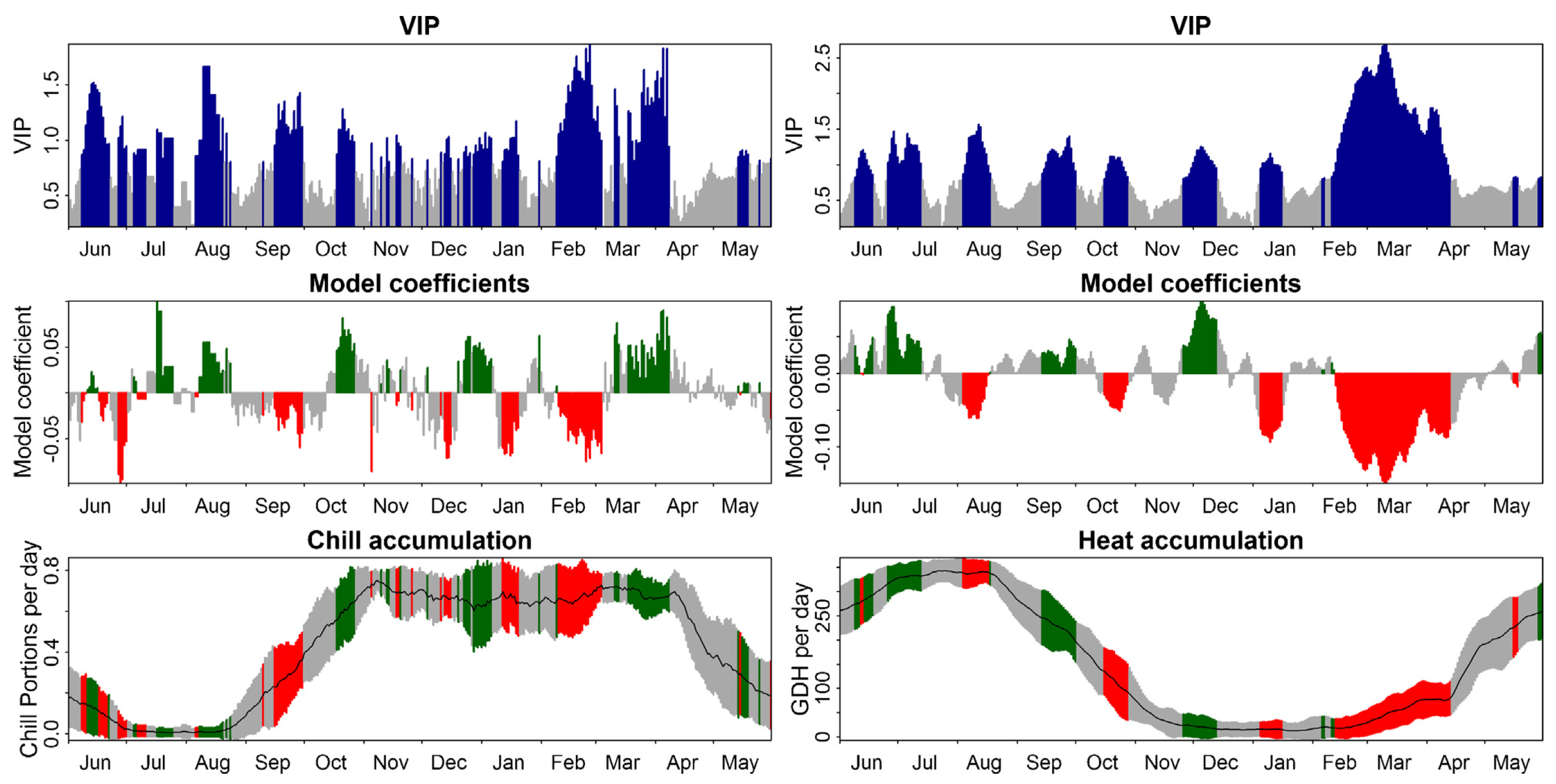
In California, where winters are even warmer, the chilling period for walnuts was evident both from raw temperature data and when using agroclimatic metrics.
The analysis again reveals a distinct chilling period, seemingly divided into two phases. The reason for this split remains unclear and may be worth further investigation. However, a clear bloom response to high chill accumulation rates is observed between mid-October and late December.
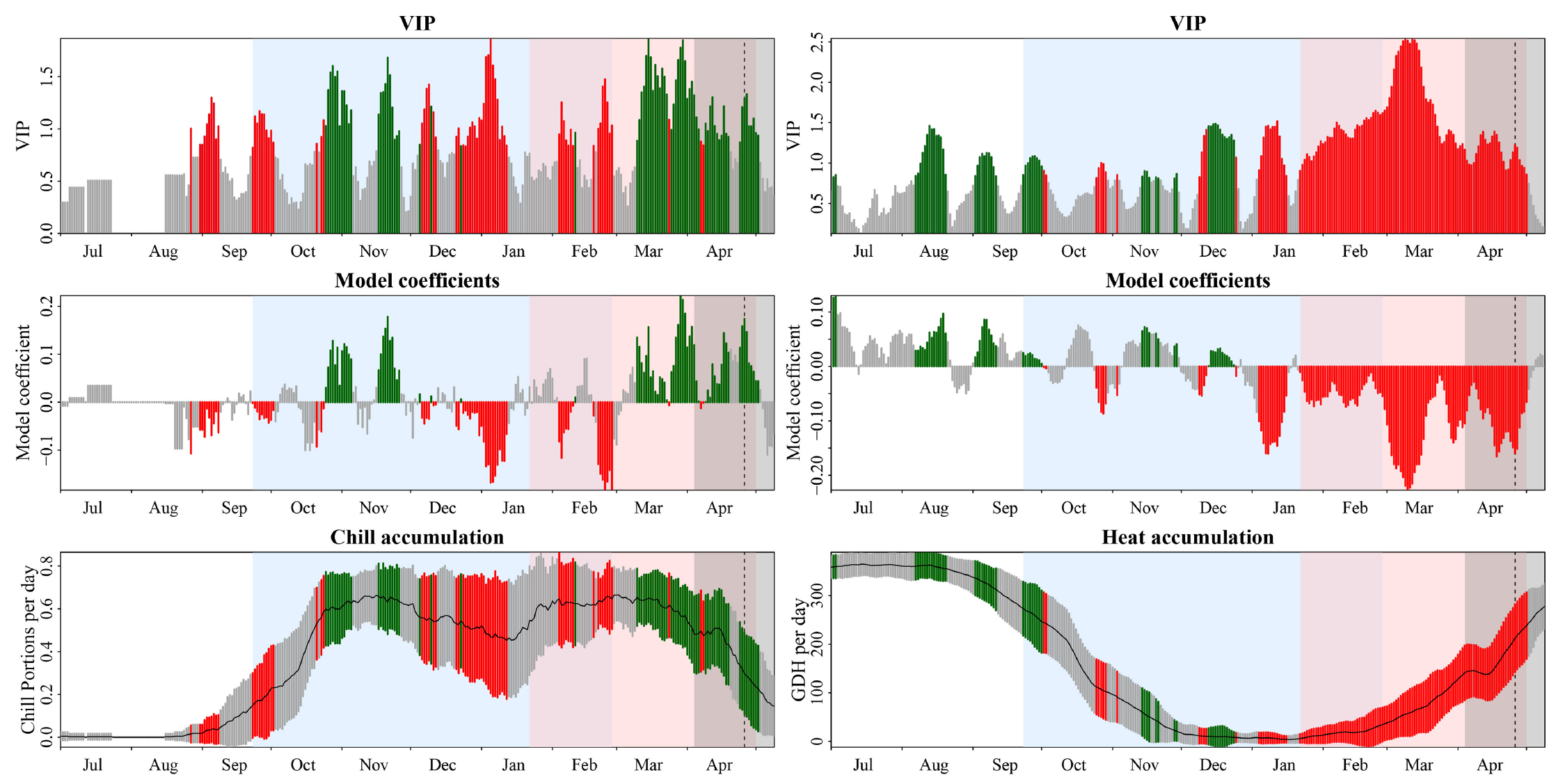
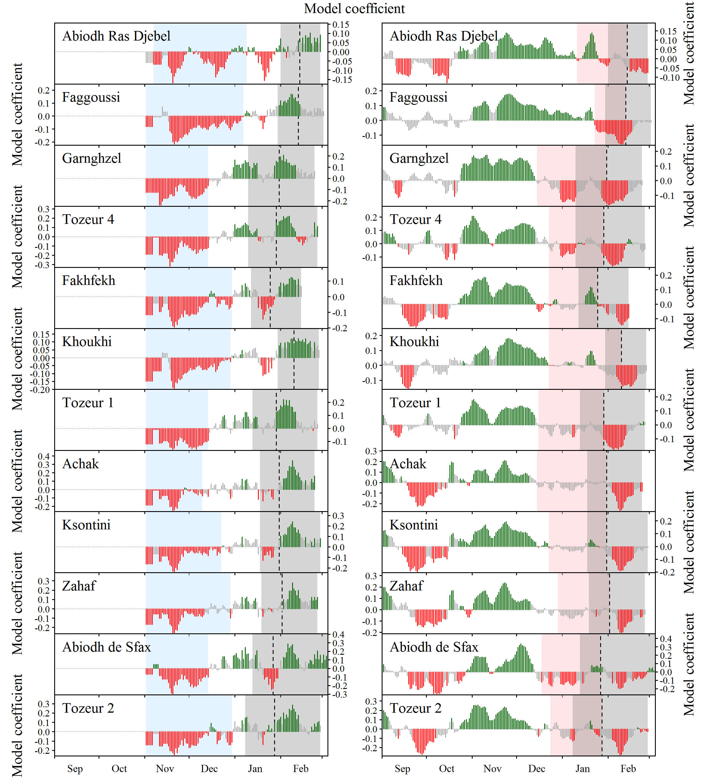
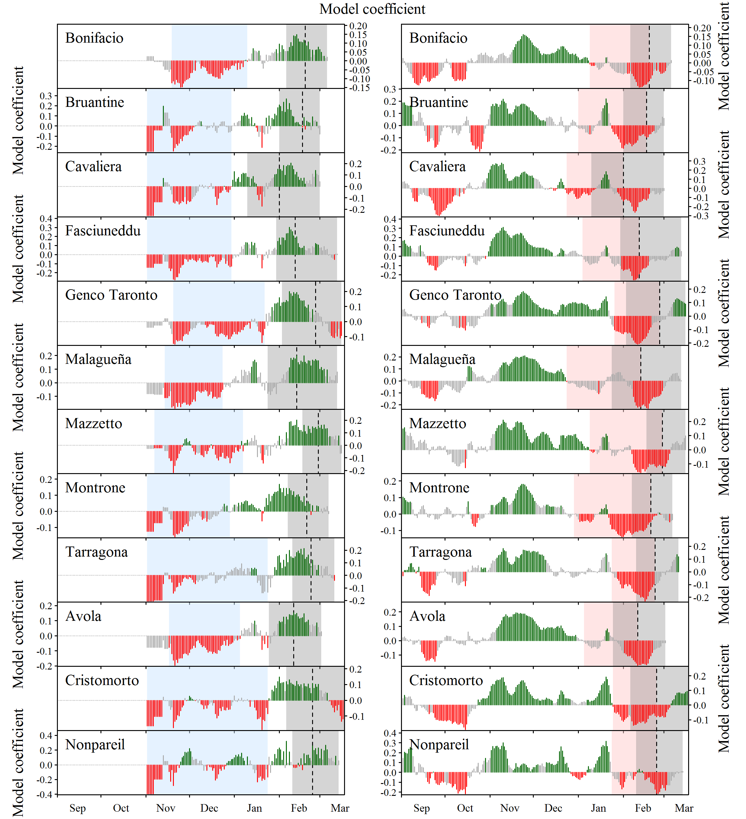
Almonds in Tunisia
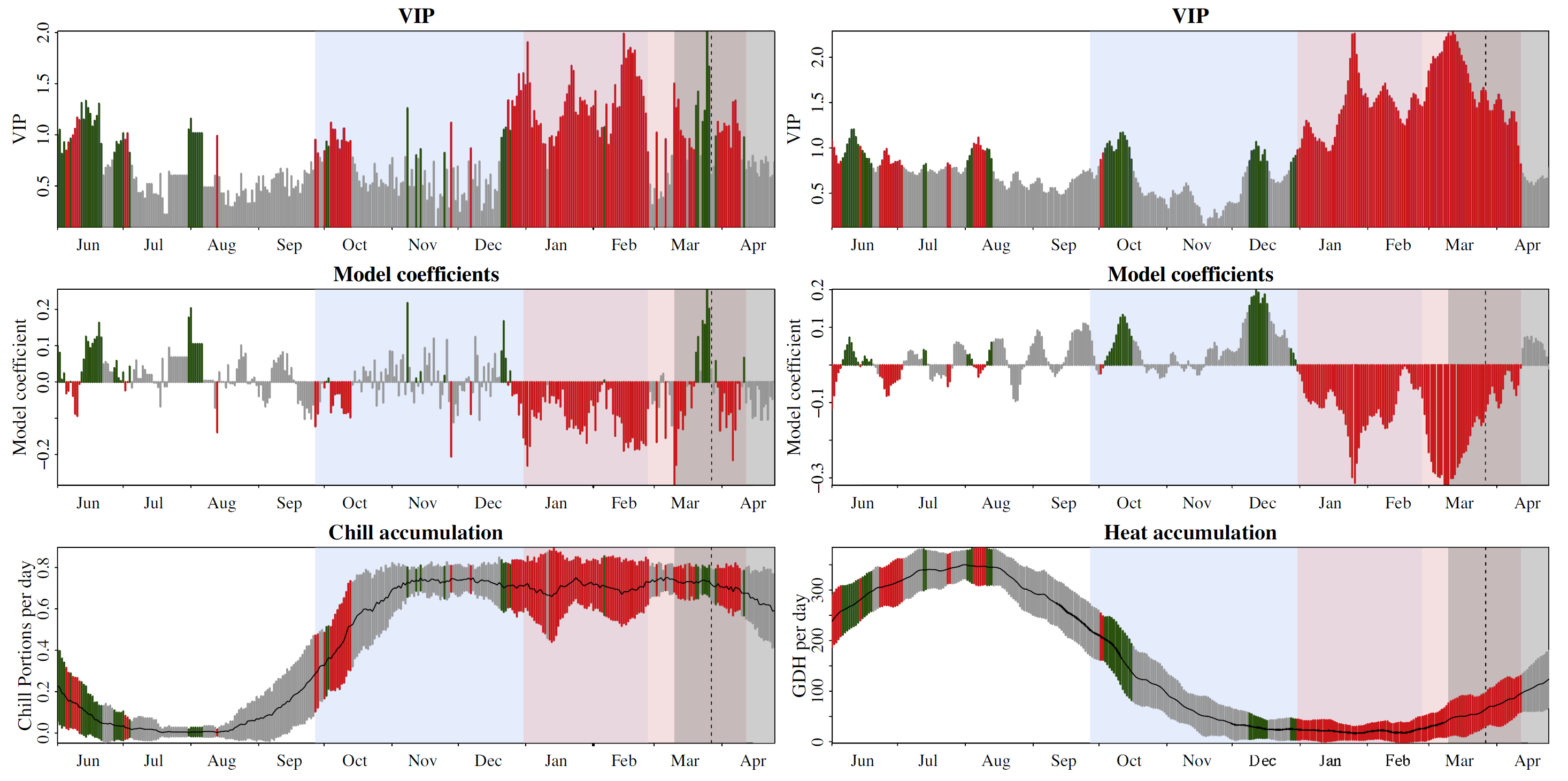
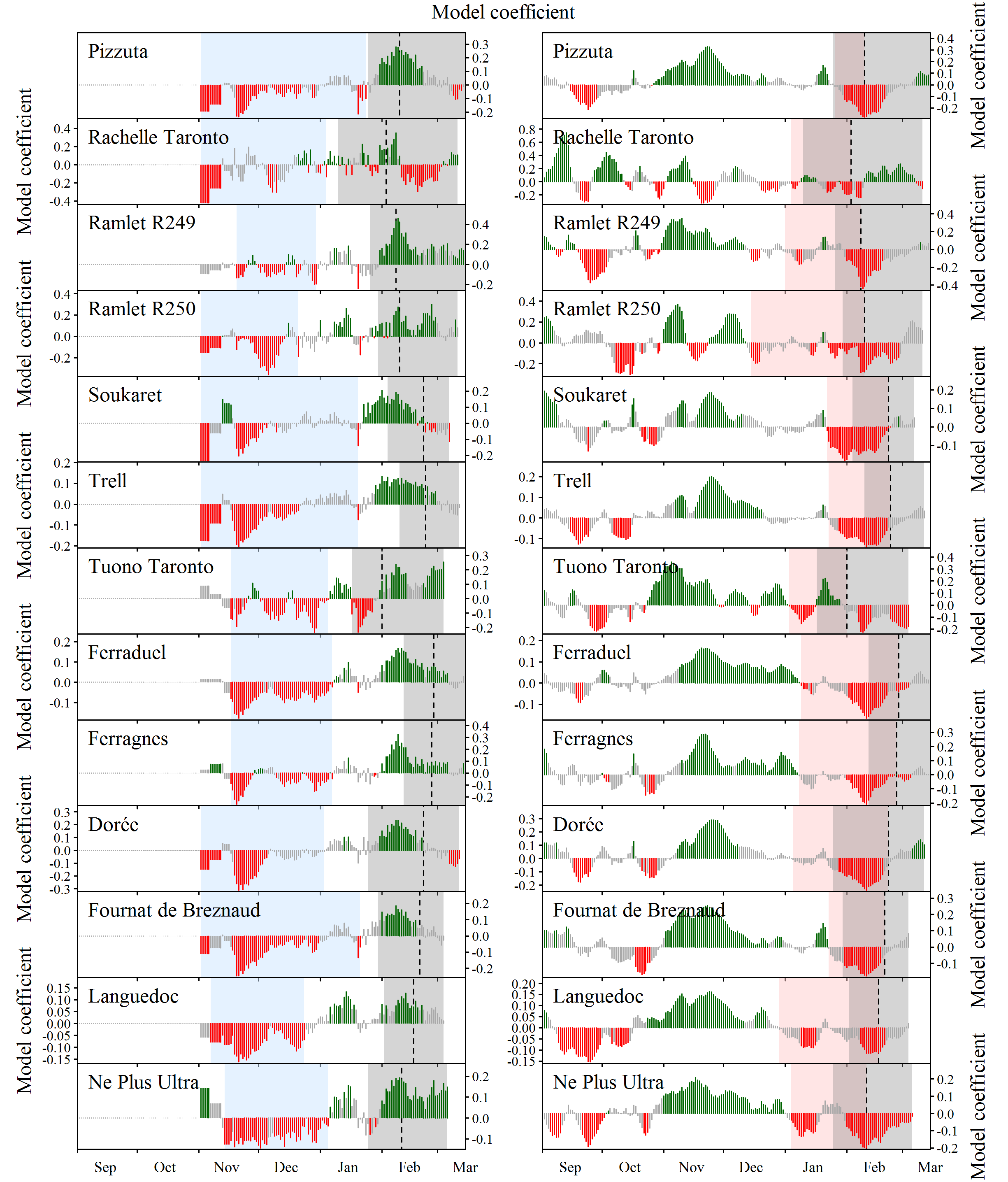
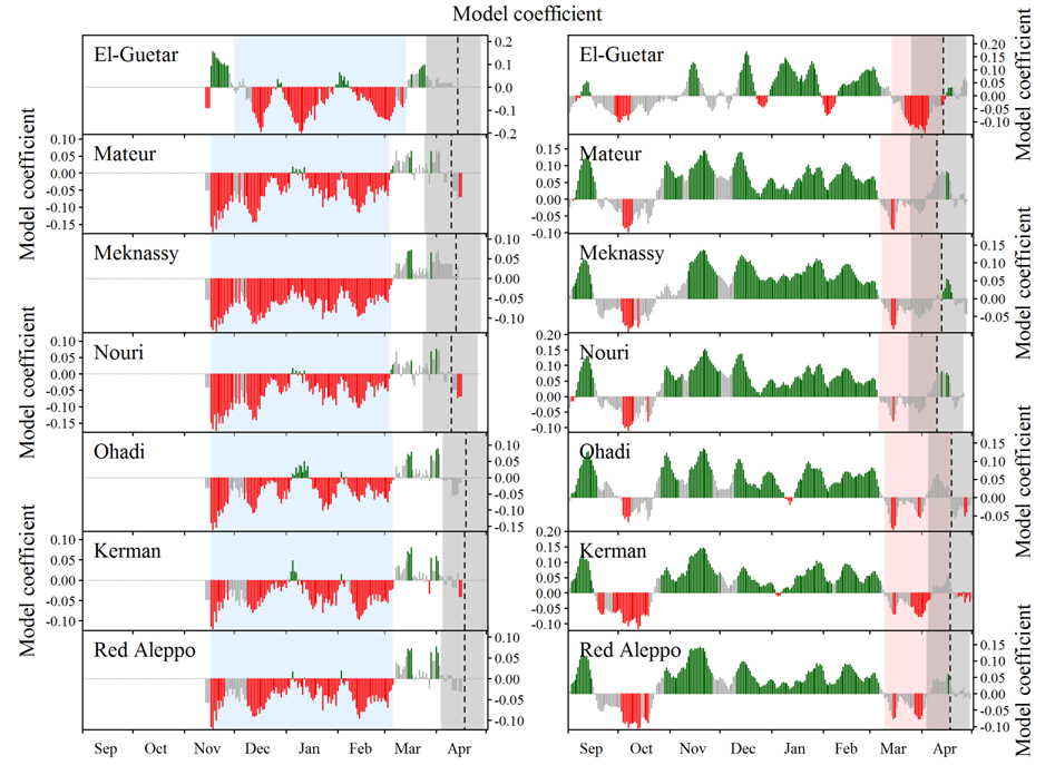
Sfax, in central Tunisia, represents an even warmer climate near the cultivation limit for temperate nut trees. A study led by Haïfa Benmoussa analyzed bloom data from 37 almond cultivars, successfully identifying both the chilling and forcing periods in nearly all cases. The following figures illustrate these findings.
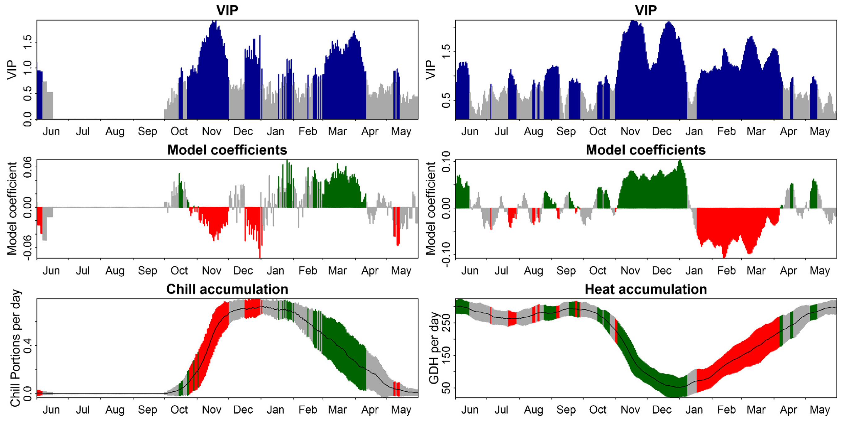
Pistachios in Tunisia
Pistachio data from the same experimental station in Sfax, Tunisia, was also analyzed. The results revealed a long chilling period with strong responses to chill accumulation rates. However, the forcing period was less distinct.
Exercises on examples of PLS regression with agroclimatic metrics
- Look across all the PLS results presented above. Can you detect a pattern in where chilling and forcing periods could be delineated clearly, and where this attempt failed?
Looking at the PLS results across different locations and crops, a clear pattern emerges regarding the delineation of chilling and forcing periods:
Chilling Period Identification:
In colder regions like Beijing, Shaanxi, and Croatia, chilling periods were generally well-defined, often spanning from late autumn to mid-winter.
In moderately cold locations like Klein-Altendorf and Brogdale Farm (UK), chilling phases were also visible, but in some cases, they appeared later than expected.
In warm locations like Sfax (Tunisia) and California, chilling periods could still be detected, but they sometimes appeared fragmented or extended over a longer time frame.
Forcing Period Identification:
In most locations, forcing periods were clearly visible and followed the expected seasonal pattern.
However, in pistachios from Sfax, the forcing phase was difficult to identify, suggesting that temperature alone may not be the primary driver of bud development in this case.
Think about possible reasons for the success or failure of PLS analysis based on agroclimatic metrics. Write down your thoughts.
Reasons for Success or Failure of PLS Analysis:
Temperature Variability:
In regions with distinct seasonal temperature changes (e.g., Beijing, Croatia), PLS was effective in identifying chilling and forcing phases
In warmer areas with mild winters (e.g., Sfax, California), chill accumulation was more gradual, leading to less distinct responses
Chilling Model Accuracy:
Different crops may respond to chilling in unique ways, and the effectiveness of PLS depends on how well the selected agroclimatic metric captures the true physiological response of the plants
The Dynamic Model often provided better results than simpler models like Chilling Hours or the Utah Model
Threshold Effects and Physiological Responses:
In some cases, the chilling phase appeared to consist of two parts, suggesting that additional factors (e.g., photoperiod, water availability) may influence dormancy release
The inability to detect a forcing period in pistachios suggests that heat accumulation alone might not fully explain bud development in this crop
Climatic Extremes:
Extremely cold winters (e.g., Beijing, Shaanxi) might lead to periods where chill accumulation is excessive, making further responses difficult to detect
In very warm climates (e.g., Sfax), chill accumulation might be insufficient in some years, causing irregular dormancy release patterns