Improvements in Phenology Models
Existing phenology models are mostly based on simple concepts of chill and heat accumulation. The Dynamic Model was developed for peaches in Israel, while the Growing Degree Hours Model originated in Utah, often without adaptation to other tree species. One crucial aspect is missing: the ability of trees to compensate for insufficient chill with additional heat.
The PhenoFlex Framework
PhenoFlex (Luedeling et al., 2021) was developed through interdisciplinary collaboration, inspired by the Dynamic Model’s origins. It integrates the Dynamic Model for chill accumulation with the Growing Degree Hours concept for heat. A sigmoidal function governs the dormancy transition, ensuring heat accumulation begins only after a critical chill threshold. Originally in R, its core code is now in C++ for better performance.
Running PhenoFlex
The chillR package now includes the PhenoFlex function, which can be run with default parameters. Before making predictions, suitable parameters should be identified. Below is a demonstration using an hourly temperature dataset from Klein-Altendorf.
library(chillR)
library(tidyverse)
CKA_weather <- read_tab("data/TMaxTMin1958-2019_patched.csv")
hourtemps <- stack_hourly_temps(CKA_weather,
                                latitude = 50.6)
A critical chilling requirement (yc) and a heat requirement (zc) are set, while all other parameters remain at their default values. The dataset is filtered for the 2009 season.
The res object contains key variables describing dormancy:
x: precursor to the dormancy-breaking factory: dormancy-breaking factor (Chill Portion)z: heat accumulation (Growing Degree Hours model)xs: ratio of formation to destruction rate ofx
The predicted bloom date is stored in res$bloomindex and can be converted to an actual date. The following plots show the development of chill accumulation (y) and heat accumulation (z) over time. Vertical lines indicate when the critical chilling requirement (blue) and heat requirement (red) are met.
DBreakDay <- res$bloomindex
seasontemps <- hourtemps$hourtemps[iSeason[[1]],]
seasontemps[,"x"] <- res$x
seasontemps[,"y"] <- res$y
seasontemps[,"z"] <- res$z
seasontemps <- add_date(seasontemps)

CR_full <- seasontemps$Date[which(seasontemps$y >= yc)[1]]
Bloom <- seasontemps$Date[which(seasontemps$z >= zc)[1]]

chillplot <- ggplot(data = seasontemps[1:DBreakDay,],
                    aes(x = Date,
                        y = y)) +
  geom_line(col = "blue",
            lwd = 1.5) +
  theme_bw(base_size = 20) +
  geom_hline(yintercept = yc,
             lty = 2,
             col = "blue",
             lwd = 1.2) +
  geom_vline(xintercept = CR_full,
             lty = 3,
             col = "blue",
             lwd = 1.2) +
  ylab("Chill accumulation (y)") +
  labs(title = "Chilling") +
  annotate("text",
           label = "Chill req. (yc)",
           x = ISOdate(2008,10,01),
           y = yc*1.1,
           col = "blue",
           size = 5)

heatplot <- ggplot(data = seasontemps[1:DBreakDay,],
                   aes(x = Date,
                       y = z)) +
  geom_line(col = "red",
            lwd = 1.5) +
  theme_bw(base_size = 20) +
  scale_y_continuous(position = "right") +
  geom_hline(yintercept = zc,
             lty = 2,
             col = "red",
             lwd = 1.2) +
  geom_vline(xintercept = CR_full,
             lty = 3,
             col = "blue",
             lwd = 1.2) +
  geom_vline(xintercept = Bloom,
             lty = 3,
             col = "red",
             lwd = 1.2) +
  ylab("Heat accumulation (z)") +
  labs(title = "Forcing") +
  annotate("text",
           label = "Heat req. (zc)",
           x = ISOdate(2008,10,01),
           y = zc*0.95,
           col = "red",
           size = 5)


library(patchwork)
chillplot + heatplot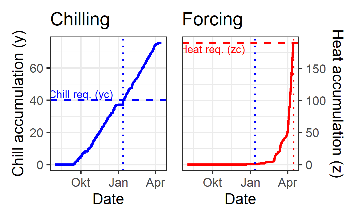
Running PhenoFlex for Multiple Years
A loop can be used to predict bloom dates for multiple years (1959–2019), outputting only the bloom date.
yc <- 40
zc <- 190
seasons <- 1959:2019

iSeason <- genSeason(hourtemps,
                     mrange = c(8, 6),
                     years = seasons)
for (sea in 1:length(seasons))
{season_data <- hourtemps$hourtemps[iSeason[[sea]], ]
 res <- PhenoFlex(temp = season_data$Temp,
                  times = c(1: length(season_data$Temp)),
                  zc = zc,
                  stopatzc = TRUE,
                  yc = yc,
                  basic_output = FALSE)
 if(sea == 1)
    results <- season_data$DATE[res$bloomindex] else
      results <- c(results,
                   season_data$DATE[res$bloomindex])}

predictions <- data.frame(Season = seasons,
                          Prediction = results)
predictions$Prediction <-
  ISOdate(2001,
          substr(predictions$Prediction, 4, 5),
          substr(predictions$Prediction, 1, 2))

ggplot(data = predictions,
       aes(x = Season,
           y = Prediction)) +
  geom_smooth() +
  geom_point() +
  ylab("Predicted bloom date") +
  theme_bw(base_size = 15)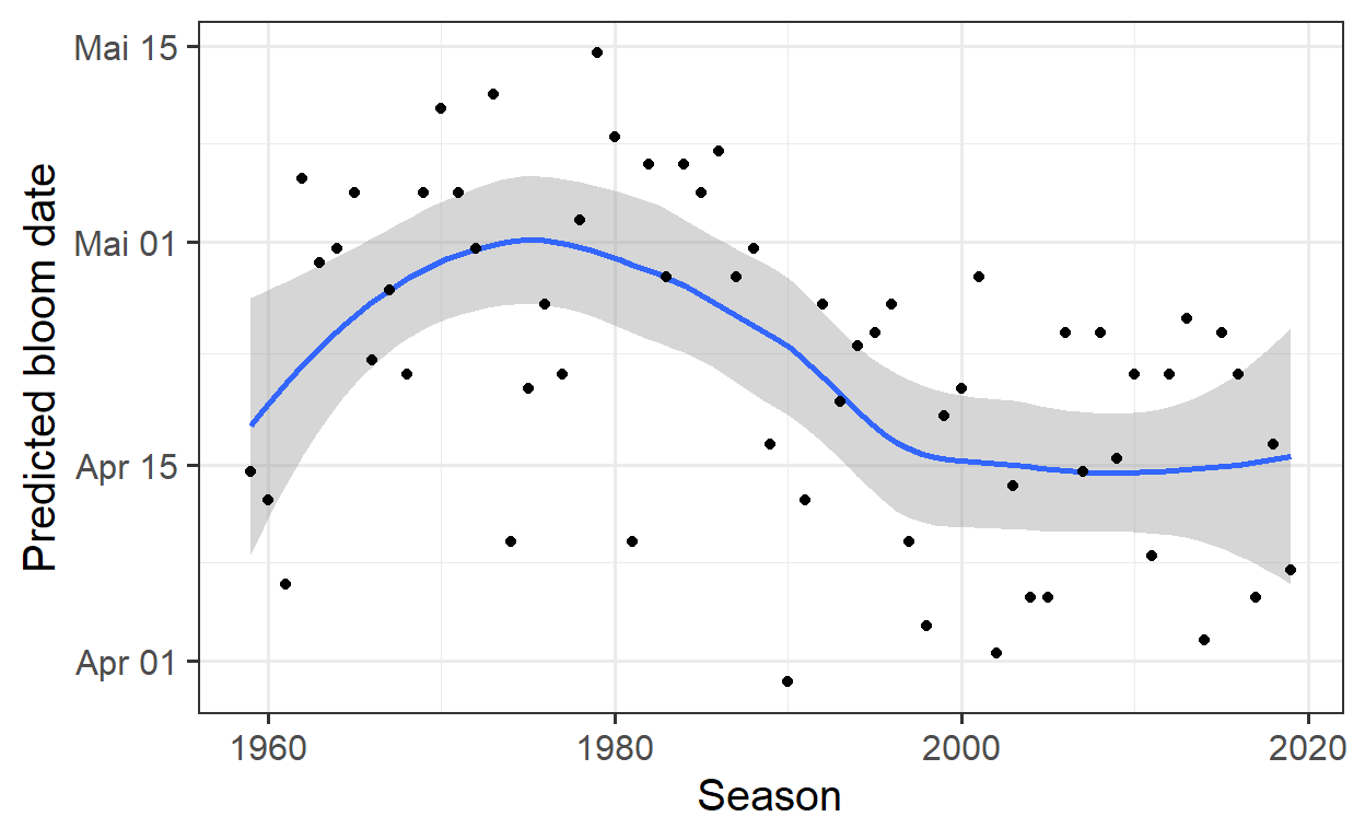
PhenoFlex can now be used to compute bloom dates but still requires parameter adjustments for specific tree cultivars. The model structure allows calibration with observed phenology data, improving prediction accuracy.
Parameterizing PhenoFlex
The PhenoFlex model is a phenological model designed to predict bloom dates based on temperature data. It consists of 12 parameters that govern chilling accumulation, heat accumulation, and dormancy-breaking processes. Since these parameters are not directly measurable from real-world biological processes, they must be estimated using computational solvers.
PhenoFlex Model Parameters
The model’s parameters define various aspects of dormancy and temperature response. Below is an overview of these parameters and their default values:
yc (Chilling requirement) – Defines the critical value at which chill accumulation ends (Default: 40)
zc (Heat requirement) – Defines the critical value at which heat accumulation ends (Default: 190)
s1 (Transition slope) – Governs the transition from chill to heat accumulation (Default: 0.5)
Tu (Optimal temperature for GDH model) – The temperature at which heat accumulation is most effective (Default: 25°C)
E0 (Activation energy for precursor formation) – A key parameter from the Dynamic Model (Default: 3372.8)
E1 (Activation energy for precursor destruction) – Represents energy needed to break down dormancy (Default: 9900.3)
A0 (Amplitude of precursor formation process) – Describes dormancy precursor production (Default: 6319.5)
A1 (Amplitude of precursor destruction process) – Determines the intensity of dormancy precursor degradation (Default: 5.94 × 10¹³)
Tf (Transition temperature for sigmoidal function) – Converts the dormancy precursor to Chill Portions (Default: 4°C)
Tc (Upper threshold for GDH model) – The maximum temperature where heat accumulation is effective (Default: 36°C)
Tb (Base temperature for GDH model) – The minimum temperature for heat accumulation (Default: 4°C)
Slope (Sigmoidal slope parameter) – Defines the rate of precursor conversion to Chill Portions (Default: 1.6)
These parameters are essential for capturing the biological response of plants to temperature variations.
Challenges in Parameter Estimation
Unlike simple regression models, PhenoFlex lacks a direct analytical solution for parameter estimation. Instead, empirical optimization techniques are needed to identify a parameter set that minimizes prediction error.
This process begins with initial parameter guesses, and plausible upper and lower bounds for each parameter are defined. The solver iteratively adjusts these values to improve predictions. However, multiple solutions can exist due to local minima in the error function, requiring multiple runs with different starting conditions.
Dataset Preparation
To fit the PhenoFlex model, historical bloom data and hourly temperature records for ‘Alexander Lucas’ pears from 1958 to 2019 were used. The data is preprocessed as follows:
Alex_first <-
  read_tab("data/Alexander_Lucas_bloom_1958_2019.csv") %>%
  select(Pheno_year, First_bloom) %>%
  mutate(Year = as.numeric(substr(First_bloom, 1, 4)),
         Month = as.numeric(substr(First_bloom, 5, 6)),
         Day = as.numeric(substr(First_bloom, 7, 8))) %>%
  make_JDay() %>%
  select(Pheno_year, JDay) %>%
  rename(Year = Pheno_year,
         pheno = JDay)

hourtemps <-
  read_tab("data/TMaxTMin1958-2019_patched.csv") %>%
  stack_hourly_temps(latitude = 50.6)
Defining Initial Parameter Sets
Before fitting the model, initial parameter values, along with their upper and lower limits, must be set:
# here's the order of the parameters (from the helpfile of the
# PhenoFlex_GDHwrapper function)
#          yc,  zc,  s1, Tu,    E0,      E1,     A0,         A1,   Tf, Tc, Tb,  slope
par <-   c(40, 190, 0.5, 25, 3372.8,  9900.3, 6319.5,
           5.939917e13,  4, 36,  4,  1.60)
upper <- c(41, 200, 1.0, 30, 4000.0, 10000.0, 7000.0,
           6.e13, 10, 40, 10, 50.00)
lower <- c(38, 180, 0.1, 0 , 3000.0,  9000.0, 6000.0,
           5.e13,  0,  0,  0,  0.05)
Since some parameters describe hypothetical biological processes, their estimation remains difficult. The activation energies (E0, E1) and amplitudes (A0, A1) in particular do not have well-defined values in literature.
Model Fitting Using Simulated Annealing
The Simulated Annealing algorithm is used to optimize the parameters. The process is as follows:
Generate a season list based on hourly temperature data.
Use the
phenologyFitterfunction to adjust the parameters iteratively.Run the solver for 1000 iterations to ensure convergence.
SeasonList <- genSeasonList(hourtemps$hourtemps,
                            mrange = c(8, 6),
                            years = c(1959:2019))

Fit_res <-
  phenologyFitter(par.guess = par,
                  modelfn = PhenoFlex_GDHwrapper,
                  bloomJDays = Alex_first$pheno[which(Alex_first$Year > 1958)],
                  SeasonList = SeasonList,
                  lower = lower,
                           upper = upper,
                           control = list(smooth = FALSE,
                                          verbose = FALSE,
                                          maxit = 1000,
                                          nb.stop.improvement = 5))

Alex_par <- Fit_res$par

write.csv(Alex_par,
          "data/PhenoFlex_parameters_Alexander_Lucas.csv")
Model Performance and Error Analysis
After fitting, the model’s predictions are compared with actual bloom dates:
Alex_par <-
  read_tab("data/PhenoFlex_parameters_Alexander_Lucas.csv")[,2]

SeasonList <- genSeasonList(hourtemps$hourtemps,
                            mrange = c(8, 6),
                            years = c(1959:2019))

Alex_PhenoFlex_predictions <- Alex_first[which(Alex_first$Year > 1958),]

for(y in 1:length(Alex_PhenoFlex_predictions$Year))
   Alex_PhenoFlex_predictions$predicted[y] <-
    PhenoFlex_GDHwrapper(SeasonList[[y]],
                         Alex_par)

Alex_PhenoFlex_predictions$Error <-
  Alex_PhenoFlex_predictions$predicted -
  Alex_PhenoFlex_predictions$pheno

RMSEP(Alex_PhenoFlex_predictions$predicted,
      Alex_PhenoFlex_predictions$pheno)
[1] 6.146689mean(Alex_PhenoFlex_predictions$Error)[1] 1.030738Visualization
The model’s performance is visualized using scatter plots and histograms:
ggplot(Alex_PhenoFlex_predictions,
       aes(x = pheno,
           y = predicted)) +
  geom_point() +
  geom_abline(intercept = 0,
              slope = 1) +
  theme_bw(base_size = 15) +
  xlab("Observed bloom date (Day of the year)") +
  ylab("Predicted bloom date (Day of the year)") +
  ggtitle("Predicted vs. observed bloom dates")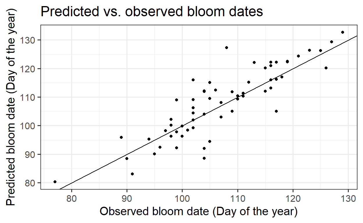
ggplot(Alex_PhenoFlex_predictions,
       aes(Error)) +
  geom_histogram() +
  ggtitle("Distribution of prediction errors")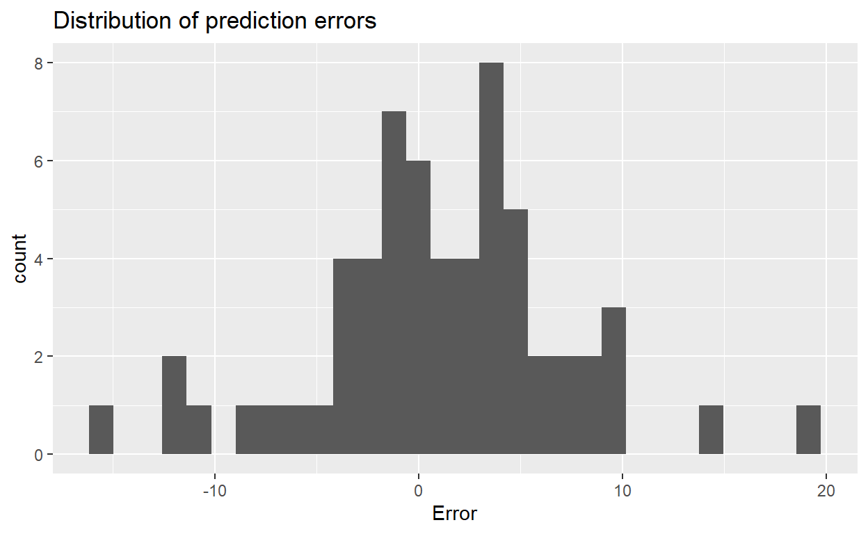
Conclusions
The PhenoFlex framework successfully predicted bloom dates for ‘Alexander Lucas’ pears in Klein-Altendorf, with errors normally distributed and evenly spread across all bloom dates. This suggests the model is reliable for both early and late blooming.
The model’s accuracy makes it a promising tool for predicting phenology under future climate conditions, outperforming previous models that lacked integration of current temperature response knowledge during dormancy.
Exercises on the PhenoFlex model
- Parameterize the
PhenoFlexmodel for `Roter Boskoop’ apples.
# Use Roter Boskoop dataset to fit the PhenoFlex model
RB_first <-
  read_tab("data/Roter_Boskoop_bloom_1958_2019.csv") %>%
  select(Pheno_year, First_bloom) %>%
  mutate(Year = as.numeric(substr(First_bloom, 1, 4)),
         Month = as.numeric(substr(First_bloom, 5, 6)),
         Day = as.numeric(substr(First_bloom, 7, 8))) %>%
  make_JDay() %>%
  select(Pheno_year, JDay) %>%
  rename(Year = Pheno_year,
         pheno = JDay)

hourtemps <-
  read_tab("data/TMaxTMin1958-2019_patched.csv") %>%
  stack_hourly_temps(latitude = 50.6)

# Parameter selection
par <- c(40, 190, 0.5, 25, 3372.8, 9900.3, 6319.5,
         5.939917e13, 4, 36, 4, 1.60)

upper <- c(41, 200, 1.0, 30, 4000.0, 10000.0, 7000.0,
           6.e13, 10, 40, 10, 50.00)

lower <- c(38, 180, 0.1, 0, 3000.0, 9000.0, 6000.0,
           5.e13, 0, 0, 0, 0.05)

# Generate season list for model fitting
SeasonList <- genSeasonList(hourtemps$hourtemps,
                            mrange = c(8, 6),
                            years = c(1959:2019))

# Fit model using phenologyFitter
Fit_res <-
  phenologyFitter(par.guess = par,
                  modelfn = PhenoFlex_GDHwrapper,
                  bloomJDays = RB_first$pheno[which(RB_first$Year >= 1958)],
                  SeasonList = SeasonList,
                  lower = lower,
                  upper = upper,
                  control = list(smooth = FALSE,
                                 verbose = FALSE,
                                 maxit = 1000,
                                 nb.stop.improvement = 5))
# Save fitted parameters
RB_par <- Fit_res$par

write.csv(RB_par,
"data/PhenoFlex_parameters_Roter_Boskoop.csv")- Produce plots of predicted vs. observed bloom dates and distribution of prediction errors.
RB_PhenoFlex_predictions <- RB_first[which(RB_first$Year > 1958),]
for(y in 1:length(RB_PhenoFlex_predictions$Year))
   RB_PhenoFlex_predictions$predicted[y] <-
    PhenoFlex_GDHwrapper(SeasonList[[y]],
                         RB_par)

RB_PhenoFlex_predictions$Error <-
  RB_PhenoFlex_predictions$predicted -
  RB_PhenoFlex_predictions$pheno

# Predicted vs. observed bloom dates
ggplot(RB_PhenoFlex_predictions,
       aes(x = pheno,
           y = predicted)) +
  geom_point() +
  geom_abline(intercept = 0,
              slope = 1) +
  theme_bw(base_size = 15) +
  xlab("Observed bloom date (Day of the year)") +
  ylab("Predicted bloom date (Day of the year)") +
  ggtitle("Predicted vs. observed bloom dates")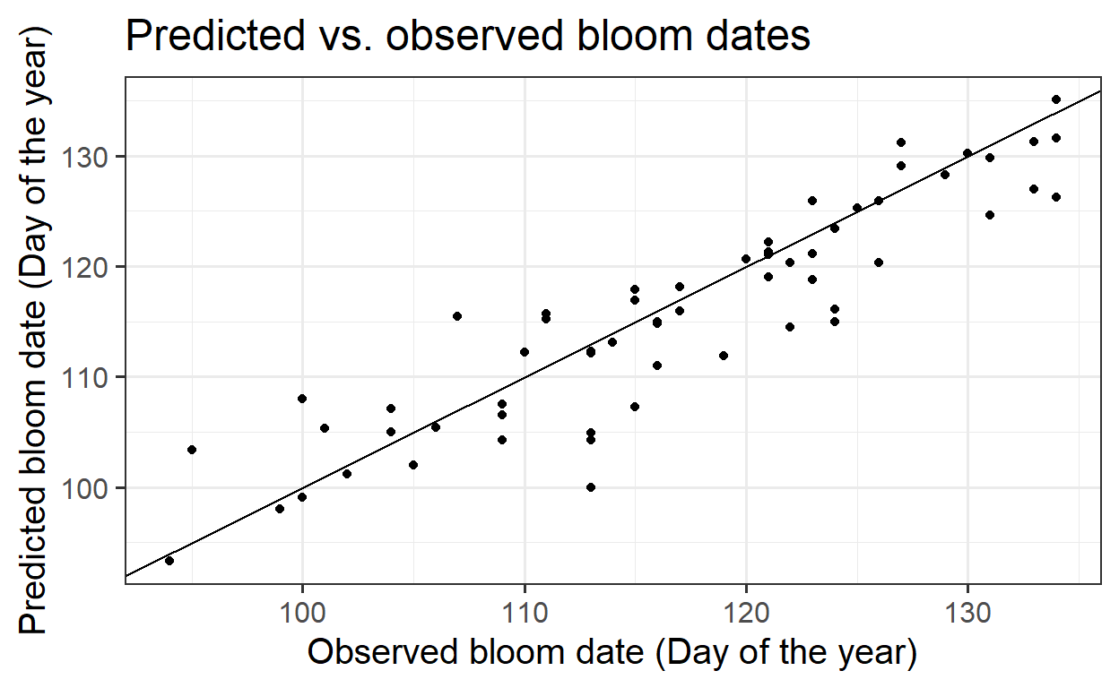
# Distribution of prediction errors
ggplot(RB_PhenoFlex_predictions,
       aes(Error)) +
  geom_histogram() +
  ggtitle("Distribution of prediction errors")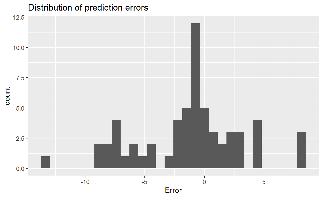
- Compute the model performance metrics RMSEP, mean error and mean absolute error.
# RMSEP
RMSEP(RB_PhenoFlex_predictions$predicted,
      RB_PhenoFlex_predictions$pheno)
[1] 4.52457# Mean Error
mean(RB_PhenoFlex_predictions$Error)[1] -1.23125