Jacqueline Wingen: Some useful tools in R

An evolving language - and a lifelong learning process

The R universe is continuously evolving, offering more than just its original base functions. Over time, modern tools and more elegant programming styles have become integral. In the upcoming chapters, we will introduce some of these new tools, along with the basics required to use them effectively.

The `tidyverse`

Many of the tools introduced here come from the tidyverse – a collection of packages developed by Hadley Wickham and his team. This collection offers numerous ways to improve programming skills. In this book, only the functions that are directly used will be covered. A major advantage of the tidyverse is that with a single command – library(tidyverse) – all functions in the package collection become available.

The `ggplot2` package

The ggplot2 package, first released by Hadley Wickham in 2007, has become one of the most popular R packages because it significantly simplifies the creation of attractive graphics. The package history can be found here, and an introduction with links to various tutorials is available here.

The `tibble` package

A tibble is an enhanced version of a data.frame offering several improvements. The most notable improvement is that tibbles avoid the common data.frame behavior of unexpectedly converting strings into factors. Although tibbles are relatively new here, they will be used throughout the rest of the book.

To create a tibble from a regular data.frame (or a similar structure), the as_tibble command can be used:

library(tidyverse)

dat <- data.frame(a = c(1, 2, 3), b = c(4, 5, 6))
d <- as_tibble(dat)
d

# A tibble: 3 × 2
      a     b
  <dbl> <dbl>
1     1     4
2     2     5
3     3     6

The `magrittr` package - pipes

Magrittr helps organize steps applied to the same dataset by using the pipe operator %>%. This operator links multiple operations on a data structure, such as a tibble, making it easier to perform tasks like calculating the sum of all numbers in the dataset:

d %>% sum()

[1] 21

After the pipe operator %>%, the next function automatically takes the piped-in data as its first input, so it’s unnecessary to specify it explicitly. Additional commands can be chained by adding more pipes, allowing for building more complex workflows, as shown in examples later.

The `tidyr` package

The tidyr package offers helpful functions for organizing data. The KA_weather dataset from chillR will be used here to illustrate some of these functions:

library(chillR)

KAw <- as_tibble(KA_weather[1:10,])
KAw

# A tibble: 10 × 5
    Year Month   Day  Tmax  Tmin
   <int> <int> <int> <dbl> <dbl>
 1  1998     1     1   8.2   5.1
 2  1998     1     2   9.1   5  
 3  1998     1     3  10.4   3.3
 4  1998     1     4   8.4   4.5
 5  1998     1     5   7.7   4.5
 6  1998     1     6   8.1   4.4
 7  1998     1     7  12     6.9
 8  1998     1     8  11.2   8.6
 9  1998     1     9  13.9   8.5
10  1998     1    10  14.5   3.6

`pivot_longer`

The pivot_longer function reshapes data from separate columns (like Tmin and Tmax) into individual rows. This transformation is often necessary for tasks like plotting data with the ggplot2 package. The function can be combined with a pipe for a streamlined workflow:

KAwlong <- KAw %>% pivot_longer(cols = Tmax:Tmin)
KAwlong

# A tibble: 20 × 5
    Year Month   Day name  value
   <int> <int> <int> <chr> <dbl>
 1  1998     1     1 Tmax    8.2
 2  1998     1     1 Tmin    5.1
 3  1998     1     2 Tmax    9.1
 4  1998     1     2 Tmin    5  
 5  1998     1     3 Tmax   10.4
 6  1998     1     3 Tmin    3.3
 7  1998     1     4 Tmax    8.4
 8  1998     1     4 Tmin    4.5
 9  1998     1     5 Tmax    7.7
10  1998     1     5 Tmin    4.5
11  1998     1     6 Tmax    8.1
12  1998     1     6 Tmin    4.4
13  1998     1     7 Tmax   12  
14  1998     1     7 Tmin    6.9
15  1998     1     8 Tmax   11.2
16  1998     1     8 Tmin    8.6
17  1998     1     9 Tmax   13.9
18  1998     1     9 Tmin    8.5
19  1998     1    10 Tmax   14.5
20  1998     1    10 Tmin    3.6

`pivot_wider`

The pivot_wider function allows for the opposite transformation of pivot_longer, converting rows back into separate columns:

KAwwide <- KAwlong %>% pivot_wider(names_from = name) 
KAwwide

# A tibble: 10 × 5
    Year Month   Day  Tmax  Tmin
   <int> <int> <int> <dbl> <dbl>
 1  1998     1     1   8.2   5.1
 2  1998     1     2   9.1   5  
 3  1998     1     3  10.4   3.3
 4  1998     1     4   8.4   4.5
 5  1998     1     5   7.7   4.5
 6  1998     1     6   8.1   4.4
 7  1998     1     7  12     6.9
 8  1998     1     8  11.2   8.6
 9  1998     1     9  13.9   8.5
10  1998     1    10  14.5   3.6

`select`

The select function allows users to choose a subset of columns from a data.frame or tibble:

KAw %>% select(c(Month, Day, Tmax))

# A tibble: 10 × 3
   Month   Day  Tmax
   <int> <int> <dbl>
 1     1     1   8.2
 2     1     2   9.1
 3     1     3  10.4
 4     1     4   8.4
 5     1     5   7.7
 6     1     6   8.1
 7     1     7  12  
 8     1     8  11.2
 9     1     9  13.9
10     1    10  14.5

`filter`

The filter function reduces a data.frame or tibble to just the rows that fulfill certain conditions:

KAw %>% filter(Tmax > 10)

# A tibble: 5 × 5
   Year Month   Day  Tmax  Tmin
  <int> <int> <int> <dbl> <dbl>
1  1998     1     3  10.4   3.3
2  1998     1     7  12     6.9
3  1998     1     8  11.2   8.6
4  1998     1     9  13.9   8.5
5  1998     1    10  14.5   3.6

`mutate`

The mutate function is essential for creating, modifying, and deleting columns in a data.frame or tibble. For example, it can be used to add new columns, such as converting Tmin and Tmax to Kelvin:

KAw_K <- KAw %>% mutate(Tmax_K = Tmax + 273.15, Tmin_K = Tmin + 273.15)
KAw_K

# A tibble: 10 × 7
    Year Month   Day  Tmax  Tmin Tmax_K Tmin_K
   <int> <int> <int> <dbl> <dbl>  <dbl>  <dbl>
 1  1998     1     1   8.2   5.1   281.   278.
 2  1998     1     2   9.1   5     282.   278.
 3  1998     1     3  10.4   3.3   284.   276.
 4  1998     1     4   8.4   4.5   282.   278.
 5  1998     1     5   7.7   4.5   281.   278.
 6  1998     1     6   8.1   4.4   281.   278.
 7  1998     1     7  12     6.9   285.   280.
 8  1998     1     8  11.2   8.6   284.   282.
 9  1998     1     9  13.9   8.5   287.   282.
10  1998     1    10  14.5   3.6   288.   277.

To delete the columns created with mutate, you can set them to NULL:

KAw_K %>% mutate(Tmin_K = NULL, Tmax_K = NULL)

# A tibble: 10 × 5
    Year Month   Day  Tmax  Tmin
   <int> <int> <int> <dbl> <dbl>
 1  1998     1     1   8.2   5.1
 2  1998     1     2   9.1   5  
 3  1998     1     3  10.4   3.3
 4  1998     1     4   8.4   4.5
 5  1998     1     5   7.7   4.5
 6  1998     1     6   8.1   4.4
 7  1998     1     7  12     6.9
 8  1998     1     8  11.2   8.6
 9  1998     1     9  13.9   8.5
10  1998     1    10  14.5   3.6

Next, the original temperature values will be replaced directly with their corresponding Kelvin values:

KAw %>% mutate(Tmin = Tmin + 273.15, Tmax = Tmax + 273.15)

# A tibble: 10 × 5
    Year Month   Day  Tmax  Tmin
   <int> <int> <int> <dbl> <dbl>
 1  1998     1     1  281.  278.
 2  1998     1     2  282.  278.
 3  1998     1     3  284.  276.
 4  1998     1     4  282.  278.
 5  1998     1     5  281.  278.
 6  1998     1     6  281.  278.
 7  1998     1     7  285.  280.
 8  1998     1     8  284.  282.
 9  1998     1     9  287.  282.
10  1998     1    10  288.  277.

`arrange`

The arrange function sorts data in data.frames or tibbles:

KAw %>% arrange(Tmax, Tmin)

# A tibble: 10 × 5
    Year Month   Day  Tmax  Tmin
   <int> <int> <int> <dbl> <dbl>
 1  1998     1     5   7.7   4.5
 2  1998     1     6   8.1   4.4
 3  1998     1     1   8.2   5.1
 4  1998     1     4   8.4   4.5
 5  1998     1     2   9.1   5  
 6  1998     1     3  10.4   3.3
 7  1998     1     8  11.2   8.6
 8  1998     1     7  12     6.9
 9  1998     1     9  13.9   8.5
10  1998     1    10  14.5   3.6

It can also sort in descending order:

KAw %>% arrange(desc(Tmax), Tmin)

# A tibble: 10 × 5
    Year Month   Day  Tmax  Tmin
   <int> <int> <int> <dbl> <dbl>
 1  1998     1    10  14.5   3.6
 2  1998     1     9  13.9   8.5
 3  1998     1     7  12     6.9
 4  1998     1     8  11.2   8.6
 5  1998     1     3  10.4   3.3
 6  1998     1     2   9.1   5  
 7  1998     1     4   8.4   4.5
 8  1998     1     1   8.2   5.1
 9  1998     1     6   8.1   4.4
10  1998     1     5   7.7   4.5

Loops

Understanding loops is essential for efficient coding. Loops enable the repetition of operations multiple times without needing to retype or copy-paste code. There are two primary types of loops: for loops and while loops.

For loops

In a for loop, explicit instructions dictate how many times the code inside the loop should be executed, based on a vector or list of elements:

for (i in 1:3) print("Hello")

[1] "Hello"
[1] "Hello"
[1] "Hello"

This code executes the loop three times, printing “Hello” each time. A more complex example uses multiple lines inside curly brackets:

addition <- 1

for (i in 1:3)
{
  addition <- addition + 1
  print(addition)
}

[1] 2
[1] 3
[1] 4

You can also use a variable such as i in more creative ways within the loop:

names <- c("Paul", "Mary", "John")

for (i in 1:3)
{
  print(paste("Hello", names[i]))
}

[1] "Hello Paul"
[1] "Hello Mary"
[1] "Hello John"

While loops

A while loop continues until a condition is no longer met:

cond <- 5

while (cond > 0)
{
  print(cond)
  cond <- cond - 1
}

[1] 5
[1] 4
[1] 3
[1] 2
[1] 1

`apply` functions

R offers a more efficient way to perform operations on multiple elements simultaneously using functions from the apply family: apply, lapply, and sapply. These functions require two key arguments: the list of items to apply the operation to and the operation itself.

`sapply`

The sapply function is used to apply an operation to a vector:

func <- function(x) x + 1
sapply(1:5, func)

[1] 2 3 4 5 6

`lapply`

The lapply function returns a list as the output, even if the input is a vector:

lapply(1:5, func)

[[1]]
[1] 2

[[2]]
[1] 3

[[3]]
[1] 4

[[4]]
[1] 5

[[5]]
[1] 6

`apply`

The apply function is designed for arrays, allowing operations to be performed either on rows (MARGIN = 1) or columns (MARGIN = 2):

mat <- matrix(c(1, 1, 1, 2, 2, 2, 3, 3, 3), c(3, 3))
apply(mat, MARGIN = 1, sum) # sum of rows

[1] 6 6 6

apply(mat, MARGIN = 2, sum) # sum of columns

[1] 3 6 9

`Exercises` on useful R tools

Based on the Winters_hours_gaps dataset, use magrittr pipes and functions of the tidyverse to accomplish the following:

1. Convert the dataset into a tibble
1. Select only the top 10 rows of the dataset

WHG <- as_tibble(Winters_hours_gaps[1:10, ])
WHG

# A tibble: 10 × 6
    Year Month   Day  Hour Temp_gaps  Temp
   <int> <int> <int> <int>     <dbl> <dbl>
 1  2008     3     3    10      15.1  15.1
 2  2008     3     3    11      17.2  17.2
 3  2008     3     3    12      18.7  18.7
 4  2008     3     3    13      18.7  18.7
 5  2008     3     3    14      18.8  18.8
 6  2008     3     3    15      19.5  19.5
 7  2008     3     3    16      19.3  19.3
 8  2008     3     3    17      17.7  17.7
 9  2008     3     3    18      15.4  15.4
10  2008     3     3    19      12.7  12.7

1. Convert the tibble to a long format, with separate rows for Temp_gaps and Temp

To see the difference between the columns Temp_gaps and Temp, rows 279 to 302 (Julian Day 15) are used below:

WHG <- as_tibble(Winters_hours_gaps[279:302, ])
WHGlong <- WHG %>% pivot_longer(cols = Temp_gaps:Temp)
WHGlong

# A tibble: 48 × 6
    Year Month   Day  Hour name      value
   <int> <int> <int> <int> <chr>     <dbl>
 1  2008     3    15     0 Temp_gaps  6.76
 2  2008     3    15     0 Temp       6.76
 3  2008     3    15     1 Temp_gaps  6.48
 4  2008     3    15     1 Temp       6.48
 5  2008     3    15     2 Temp_gaps  5.51
 6  2008     3    15     2 Temp       5.51
 7  2008     3    15     3 Temp_gaps  6.89
 8  2008     3    15     3 Temp       6.89
 9  2008     3    15     4 Temp_gaps  6.10
10  2008     3    15     4 Temp       6.10
# ℹ 38 more rows

1. Use ggplot2 to plot Temp_gaps and Temp as facets (point or line plot)

ggplot(WHGlong, aes(Hour, value)) +
  geom_line(lwd = 1.5) +
  facet_grid(cols = vars(name)) +
  ylab("Temperature (°C)") +
  theme_bw(base_size = 15)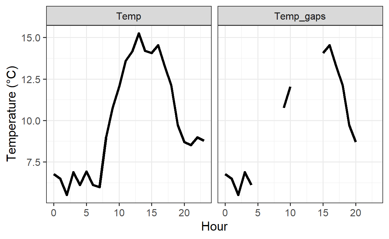

1. Convert the dataset back to the wide format

WHGwide <- WHGlong %>% pivot_wider(names_from = name)
WHGwide

# A tibble: 24 × 6
    Year Month   Day  Hour Temp_gaps  Temp
   <int> <int> <int> <int>     <dbl> <dbl>
 1  2008     3    15     0      6.76  6.76
 2  2008     3    15     1      6.48  6.48
 3  2008     3    15     2      5.51  5.51
 4  2008     3    15     3      6.89  6.89
 5  2008     3    15     4      6.10  6.10
 6  2008     3    15     5     NA     6.91
 7  2008     3    15     6     NA     6.10
 8  2008     3    15     7     NA     5.98
 9  2008     3    15     8     NA     8.99
10  2008     3    15     9     10.8  10.8 
# ℹ 14 more rows

1. Select only the following columns: Year, Month, Day and Temp

WHG %>% select(c(Year, Month, Day, Temp))

# A tibble: 24 × 4
    Year Month   Day  Temp
   <int> <int> <int> <dbl>
 1  2008     3    15  6.76
 2  2008     3    15  6.48
 3  2008     3    15  5.51
 4  2008     3    15  6.89
 5  2008     3    15  6.10
 6  2008     3    15  6.91
 7  2008     3    15  6.10
 8  2008     3    15  5.98
 9  2008     3    15  8.99
10  2008     3    15 10.8 
# ℹ 14 more rows

1. Sort the dataset by the Temp column, in descending order

WHG %>% arrange(desc(Temp))

# A tibble: 24 × 6
    Year Month   Day  Hour Temp_gaps  Temp
   <int> <int> <int> <int>     <dbl> <dbl>
 1  2008     3    15    13      NA    15.2
 2  2008     3    15    16      14.5  14.5
 3  2008     3    15    14      NA    14.2
 4  2008     3    15    12      NA    14.2
 5  2008     3    15    15      14.1  14.1
 6  2008     3    15    11      NA    13.6
 7  2008     3    15    17      13.3  13.3
 8  2008     3    15    18      12.1  12.1
 9  2008     3    15    10      12.0  12.0
10  2008     3    15     9      10.8  10.8
# ℹ 14 more rows

For the Winter_hours_gaps dataset, write a for loop to convert all temperatures (Temp column) to degrees Fahrenheit

So that the execution of the following code does not take too long, only Julian Day 15 (rows 279 to 302) is used here. To convert the entire Temp column to Fahrenheit, just omit [279:302]

Temp <- Winters_hours_gaps$Temp[279:302]

for (i in Temp)
{
  Fahrenheit <- i * 1.8 + 32 
  print(Fahrenheit)
}

[1] 44.1734
[1] 43.6712
[1] 41.9252
[1] 44.4002
[1] 42.9836
[1] 44.4452
[1] 42.9836
[1] 42.755
[1] 48.182
[1] 51.3698
[1] 53.69
[1] 56.4692
[1] 57.506
[1] 59.4446
[1] 57.5492
[1] 57.3332
[1] 58.1522
[1] 55.9058
[1] 53.8196
[1] 49.4708
[1] 47.6474
[1] 47.3342
[1] 48.182
[1] 47.7806

Execute the same operation with a function from the apply family

Here it is the same as in 2, just omit [279:302] to convert the entire Temp column

x <- Winters_hours_gaps$Temp

fahrenheit <- function(x)
  x * 1.8 + 32

sapply(x[279:302], fahrenheit)

 [1] 44.1734 43.6712 41.9252 44.4002 42.9836 44.4452 42.9836 42.7550
 [9] 48.1820 51.3698 53.6900 56.4692 57.5060 59.4446 57.5492 57.3332
[17] 58.1522 55.9058 53.8196 49.4708 47.6474 47.3342 48.1820 47.7806

Now use the tidyverse function mutate to achieve the same outcome

WHG_F <- WHG %>% mutate(Temp_F = Temp * 1.8 + 32)
WHG_F

# A tibble: 24 × 7
    Year Month   Day  Hour Temp_gaps  Temp Temp_F
   <int> <int> <int> <int>     <dbl> <dbl>  <dbl>
 1  2008     3    15     0      6.76  6.76   44.2
 2  2008     3    15     1      6.48  6.48   43.7
 3  2008     3    15     2      5.51  5.51   41.9
 4  2008     3    15     3      6.89  6.89   44.4
 5  2008     3    15     4      6.10  6.10   43.0
 6  2008     3    15     5     NA     6.91   44.4
 7  2008     3    15     6     NA     6.10   43.0
 8  2008     3    15     7     NA     5.98   42.8
 9  2008     3    15     8     NA     8.99   48.2
10  2008     3    15     9     10.8  10.8    51.4
# ℹ 14 more rows

Some useful tools in R

An evolving language - and a lifelong learning process

The tidyverse

The ggplot2 package

The tibble package

The magrittr package - pipes

The tidyr package

pivot_longer

pivot_wider

select

filter

mutate

arrange