Basic Diagnostics for PhenoFlex Fit
When developing a new model, it’s easy to become overly enthusiastic and overlook potential weaknesses. This is a common issue for modelers, particularly those without proper statistical training who may not be as aware of the potential pitfalls.
To examine the PhenoFlex framework and its parameters, helper functions can be used to explore the temperature response during chilling and forcing periods.
apply_const_temp <-
  function(temp, A0, A1, E0, E1, Tf, slope, portions = 1200, deg_celsius = TRUE)
    {
  temp_vector <- rep(temp,
                     times = portions)
  res <- chillR::DynModel_driver(temp = temp_vector,
                                 A0 = A0,
                                 A1 = A1,
                                 E0 = E0,
                                 E1 = E1,
                                 Tf = Tf,
                                 slope = slope,
                                 deg_celsius = deg_celsius)
  return(res$y[length(res$y)])
}

gen_bell <- function(par,
                     temp_values = seq(-5, 20, 0.1)) {
  E0 <- par[5]
  E1 <- par[6]
  A0 <- par[7]
  A1 <- par[8]
  Tf <- par[9]
  slope <- par[12]

  y <- c()
  for(i in seq_along(temp_values)) {
    y[i] <- apply_const_temp(temp = temp_values[i],
                             A0 = A0,
                             A1 = A1,
                             E0 = E0,
                             E1 = E1,
                             Tf = Tf,
                             slope = slope)
  }
  return(invisible(y))
}

GDH_response <- function(T, par)
  {Tb <- par[11]
   Tu <- par[4]
   Tc <- par[10]
   GDH_weight <- rep(0, length(T))
   GDH_weight[which(T >= Tb & T <= Tu)] <-
     1/2 * (1 + cos(pi + pi * (T[which(T >= Tb & T <= Tu)] - Tb)/(Tu - Tb)))
   GDH_weight[which(T > Tu & T <= Tc)] <-
     (1 + cos(pi/2 + pi/2 * (T[which(T >  Tu & T <= Tc)] -Tu)/(Tc - Tu)))
  return(GDH_weight)
}
The gen_bell function generates the chilling response curve, and GDH_response illustrates the heat effectiveness curve.
These functions can be applied to the parameter set for ‘Alexander Lucas’ pears:
Alex_par <- read_tab("data/PhenoFlex_parameters_Alexander_Lucas.csv")[,2]

temp_values = seq(-5, 30, 0.1)

temp_response <- data.frame(Temperature = temp_values,
                            Chill_response = gen_bell(Alex_par,
                                                      temp_values),
                            Heat_response = GDH_response(temp_values,
                                                         Alex_par))

pivoted_response <- pivot_longer(temp_response,
                                 c(Chill_response,
                                   Heat_response))

ggplot(pivoted_response,
       aes(x = Temperature,
           y = value)) +
  geom_line(linewidth = 2,
            aes(col = name)) +
  ylab("Temperature response (arbitrary units)") +
  xlab("Temperature (°C)") +
  facet_wrap(vars(name),
             scales = "free",
             labeller =
               labeller(name = c(Chill_response = c("Chill response"),
                                     Heat_response = c("Heat response")))) +
  scale_color_manual(values = c("Chill_response" = "blue",
                                "Heat_response" = "red")) +
  theme_bw(base_size = 15) +
  theme(legend.position = "none")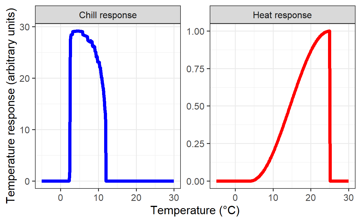
The response curves show reasonable patterns. The chilling curve peaks around 2-3°C and declines sharply after 6°C, assuming constant temperatures, which rarely occur in orchards. The heat response also appears plausible, though the final drop-off at high temperatures (30°C) may not be accurate, as such temperatures are rarely observed during dormancy.
PhenoFlex Temperature Response
In this case, temperature responses are evaluated based on daily minimum and maximum temperatures, as opposed to assuming constant temperatures. Below is the simulation process:
latitude <- 50.6

month_range <- c(10, 11, 12, 1, 2, 3)

Tmins = c(-20:20)
Tmaxs = c(-15:30)

mins <- NA
maxs <- NA
chill_eff <- NA
heat_eff <- NA
month <- NA

simulation_par <- Alex_par

for(mon in month_range)
    {days_month <- as.numeric(difftime(ISOdate(2002, mon+1, 1),
                                       ISOdate(2002, mon, 1)))
     if(mon == 12) days_month <- 31
     weather <-
       make_all_day_table(data.frame(Year = c(2002, 2002),
                                     Month = c(mon, mon),
                                     Day = c(1, days_month),
                                     Tmin = c(0, 0),
                                     Tmax = c(0, 0)))

     for(tmin in Tmins)
      for(tmax in Tmaxs)
        if(tmax >= tmin)
          {
           hourtemps <- weather %>%
             mutate(Tmin = tmin,
                    Tmax = tmax) %>%
             stack_hourly_temps(latitude = latitude) %>%
             pluck("hourtemps", "Temp")

           chill_eff <-
             c(chill_eff,
               PhenoFlex(temp = hourtemps,
                         times = c(1: length(hourtemps)),
                         A0 = simulation_par[7],
                         A1 = simulation_par[8],
                         E0 = simulation_par[5],
                         E1 = simulation_par[6],
                         Tf = simulation_par[9],
                         slope = simulation_par[12],
                         deg_celsius = TRUE,
                         basic_output = FALSE)$y[length(hourtemps)] /
                                            (length(hourtemps) / 24))

          heat_eff <-
            c(heat_eff,
              cumsum(GDH_response(hourtemps,
                                  simulation_par))[length(hourtemps)] /
                                                 (length(hourtemps) / 24))
          mins <- c(mins, tmin)
          maxs <- c(maxs, tmax)
          month <- c(month, mon)
        }
}

results <- data.frame(Month = month,
                      Tmin = mins,
                      Tmax = maxs,
                      Chill_eff = chill_eff,
                      Heat_eff = heat_eff) %>%
  filter(!is.na(Month))

write.csv(results,
          "data/model_sensitivity_PhenoFlex.csv")
Next, the results can be visualized to examine chill and heat efficiency sensitivities:
Model_sensitivities_PhenoFlex <-
  read.csv("data/model_sensitivity_PhenoFlex.csv")

CKA_weather <- read_tab("data/TMaxTMin1958-2019_patched.csv")


Chill_sensitivity_temps(Model_sensitivities_PhenoFlex,
                        CKA_weather,
                        temp_model = "Chill_eff",
                        month_range = c(10, 11, 12, 1, 2, 3),
                        Tmins = c(-20:20),
                        Tmaxs = c(-15:30),
                        legend_label = "Chill per day \n(arbitrary)") +
  ggtitle("PhenoFlex chill efficiency ('Alexander Lucas')")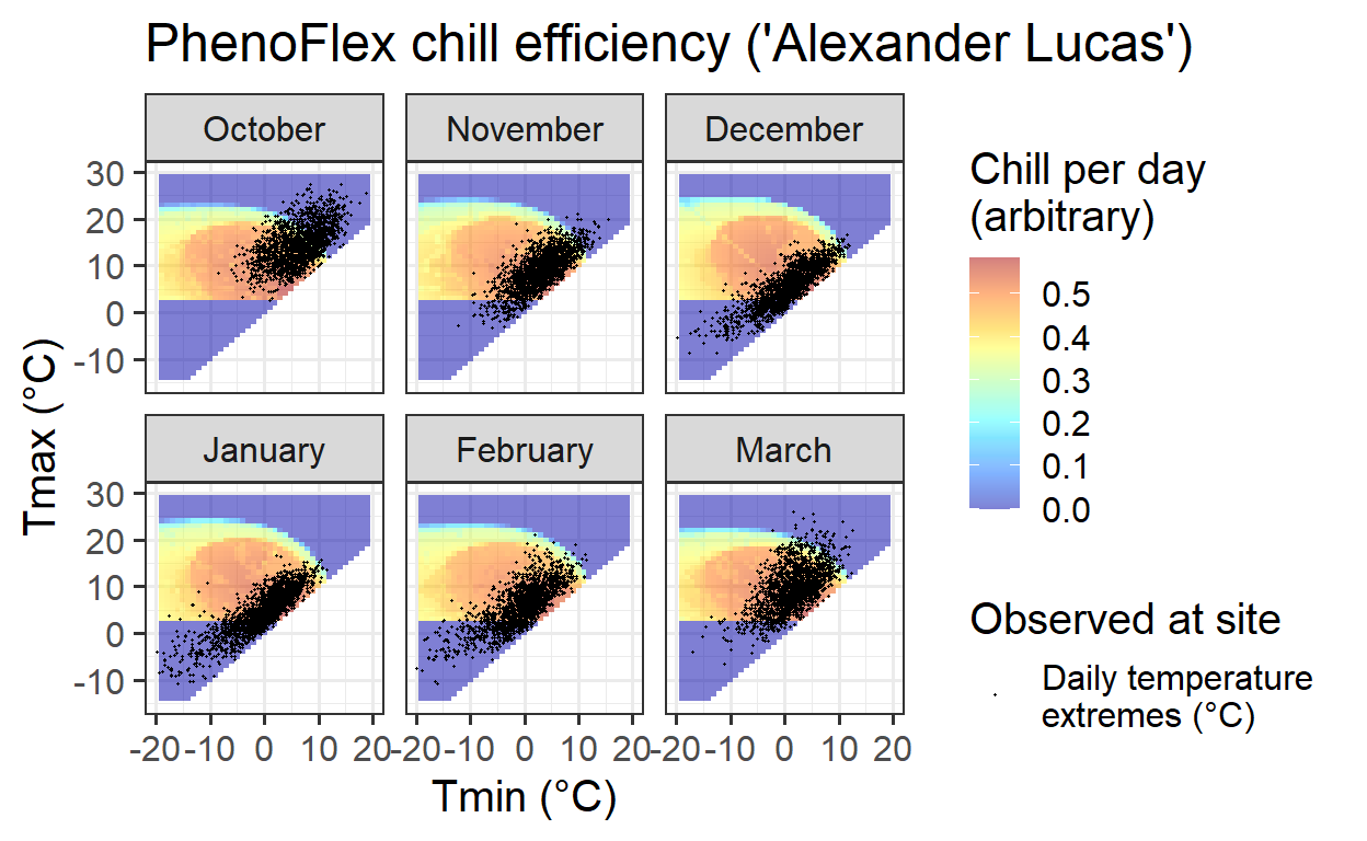
Chill_sensitivity_temps(Model_sensitivities_PhenoFlex,
                        CKA_weather,
                        temp_model = "Heat_eff",
                        month_range = c(10, 11, 12, 1, 2, 3),
                        Tmins = c(-20:20),
                        Tmaxs = c(-15:30),
                        legend_label = "Heat per day \n(arbitrary)") +
  ggtitle("PhenoFlex heat efficiency ('Alexander Lucas')")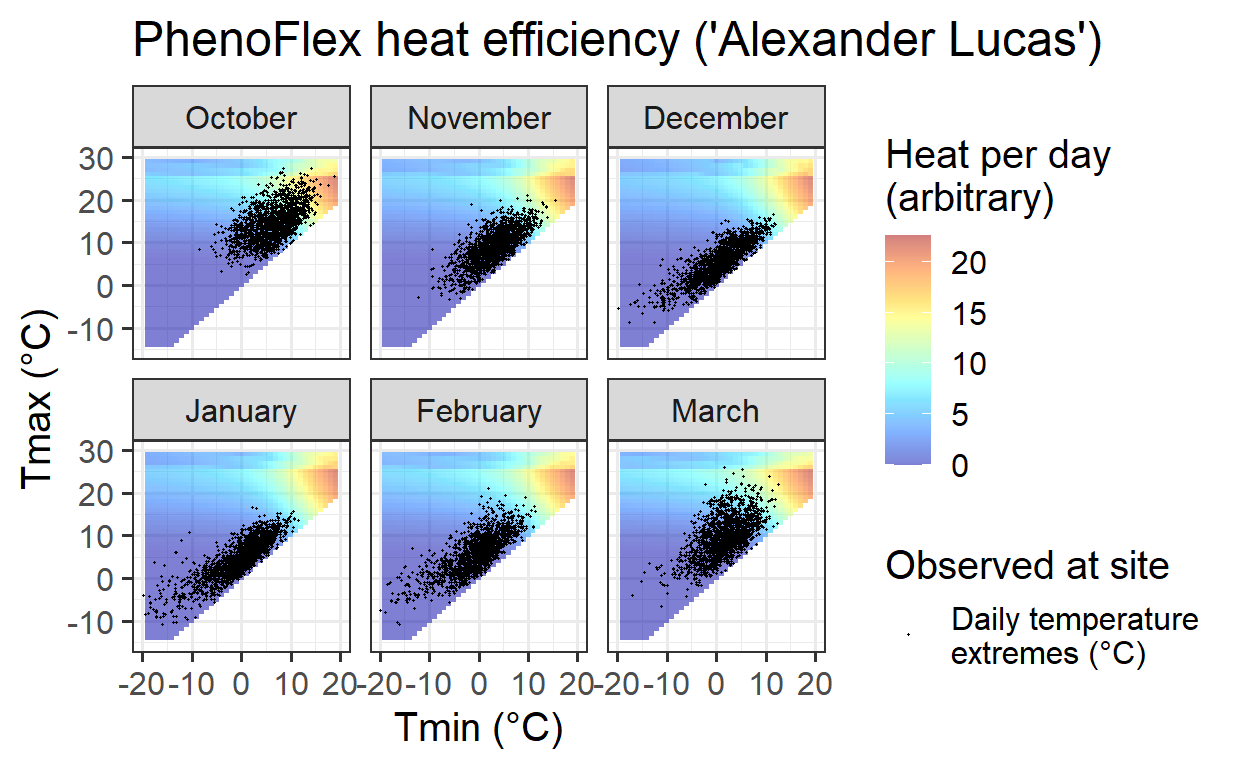
Overall Impression
Evaluating the accuracy of the PhenoFlex model remains challenging. Although the fit is good, the model should be assessed beyond predictive performance. It aligns well with existing knowledge about tree phenology during dormancy and is consistent with the parameterization derived from the data.
Caveats and Assumptions
The parameter ranges used for the model fit were quite restricted, which could have limited the model’s flexibility. Several assumptions were made, including the start date of chill accumulation and the general nature of chill and heat accumulation dynamics. Additionally, the model’s output is location- and cultivar-specific, which complicates comparisons across regions.
Outlook
The PhenoFlex model requires further testing, better guidance for parameter selection, and standardization of chill and heat units. It should also be applied across various climates to explore its potential for future phenology projections.
Exercises on basic PhenoFlex diagnostics
- Make chill and heat response plots for the ‘Roter Boskoop’
PhenoFlexmodel for the location you did the earlier analyses for.
# Evaluate temperature responses based on daily minimum and maximum temperatures
latitude <- 50.6

month_range <- c(10, 11, 12, 1, 2, 3)

Tmins = c(-20:20)
Tmaxs = c(-15:30)

mins <- NA
maxs <- NA
chill_eff <- NA
heat_eff <- NA
month <- NA

simulation_par <- RB_par

for(mon in month_range)
    {days_month <- as.numeric(difftime(ISOdate(2002, mon+1, 1),
                                       ISOdate(2002, mon, 1)))
     if(mon == 12) days_month <- 31
     weather <-
       make_all_day_table(data.frame(Year = c(2002, 2002),
                                     Month = c(mon, mon),
                                     Day = c(1, days_month),
                                     Tmin = c(0, 0),
                                     Tmax = c(0, 0)))

     for(tmin in Tmins)
      for(tmax in Tmaxs)
        if(tmax >= tmin)
          {
           hourtemps <- weather %>%
             mutate(Tmin = tmin,
                    Tmax = tmax) %>%
             stack_hourly_temps(latitude = latitude) %>%
             pluck("hourtemps", "Temp")

           chill_eff <-
             c(chill_eff,
               PhenoFlex(temp = hourtemps,
                         times = c(1: length(hourtemps)),
                         A0 = simulation_par[7],
                         A1 = simulation_par[8],
                         E0 = simulation_par[5],
                         E1 = simulation_par[6],
                         Tf = simulation_par[9],
                         slope = simulation_par[12],
                         deg_celsius = TRUE,
                         basic_output = FALSE)$y[length(hourtemps)] /
                                            (length(hourtemps) / 24))

          heat_eff <-
            c(heat_eff,
              cumsum(GDH_response(hourtemps,
                                  simulation_par))[length(hourtemps)] /
                                                 (length(hourtemps) / 24))
          mins <- c(mins, tmin)
          maxs <- c(maxs, tmax)
          month <- c(month, mon)
        }
}

results <- data.frame(Month = month,
                      Tmin = mins,
                      Tmax = maxs,
                      Chill_eff = chill_eff,
                      Heat_eff = heat_eff) %>%
  filter(!is.na(Month))

write.csv(results,
          "data/model_sensitivity_PhenoFlex_RB.csv")
# Plot chill response fo 'Roter Boskoop'
Chill_sensitivity_temps(Model_sensitivities_PhenoFlex,
CKA_weather,
temp_model = "Chill_eff",
month_range = c(10, 11, 12, 1, 2, 3),
Tmins = c(-20:20),
Tmaxs = c(-15:30),
legend_label = "Chill per day \n(arbitrary)") +
ggtitle("PhenoFlex chill efficiency ('Roter Boskoop')")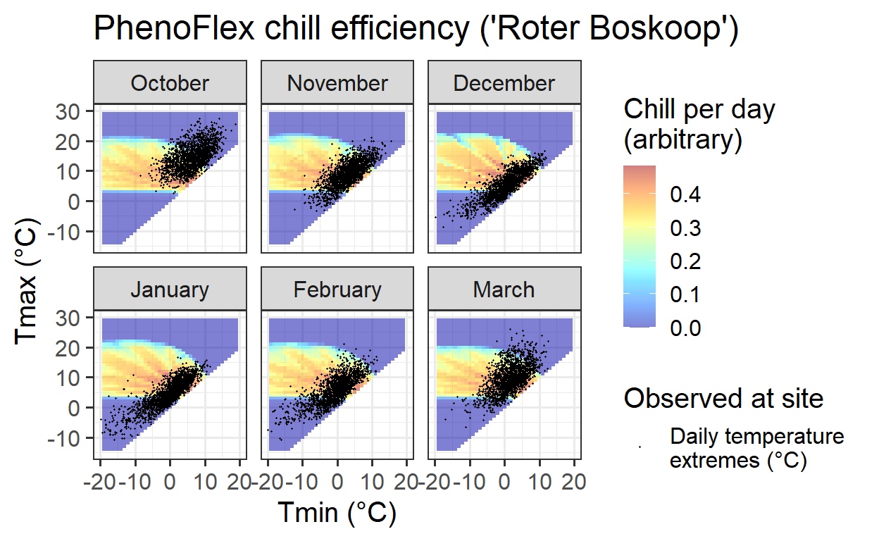
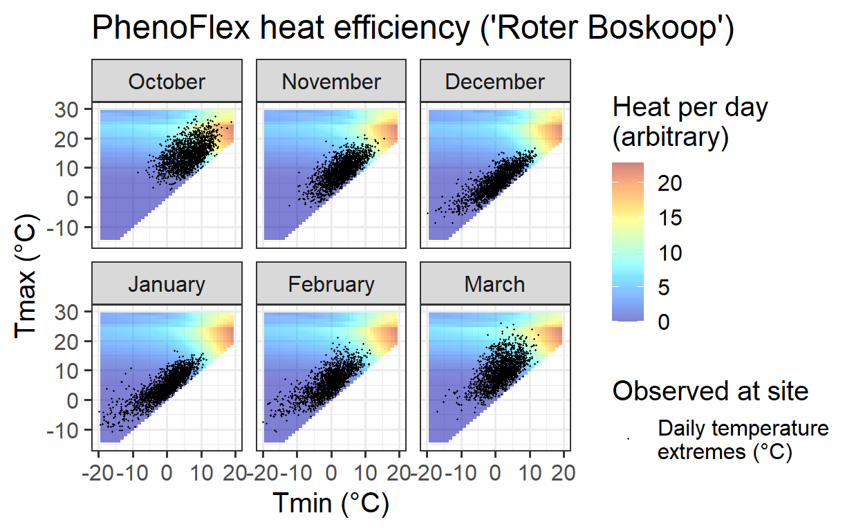
# Plot heat response of 'Roter Boskoop'
Chill_sensitivity_temps(Model_sensitivities_PhenoFlex,
                        CKA_weather,
                        temp_model = "Heat_eff",
                        month_range = c(10, 11, 12, 1, 2, 3),
                        Tmins = c(-20:20),
                        Tmaxs = c(-15:30),
                        legend_label = "Heat per day \n(arbitrary)") +
  ggtitle("PhenoFlex heat efficiency ('Roter Boskoop')")